Machine Learning for Geosciences:
Time Series and Classification (2023)
CH 0: Course Objectives
Midterm
Final
-
Overview of the machine and deep learning approaches.
-
Use unsupervised learning (K-means) to cluster crop types based on satellite imagery.
-
Use supervised learning (decision tree) to press crop types based on satellite imagery.
-
Transform satellite imagery into a machine learning-friendly data format.
-
Create a machine learning pipeline, familiarizing pre-processing data such as data normalization and outlier removal.
-
Evaluate models.
-
Conduct a midterm project using XGBoost with hyperparameter-tuning, targeting crop classification.
-
Learn mathematical methods for machine learning.
-
Overview time series analysis in machine learning, e.g., forecasting and clustering.
-
Gather satellite imagery via Google Earth Engine (GEE) into time series.
-
Transform temporal and spatial evaluation of satellite imagery in rice cultivation into time series.
-
Cluster rice-growing phases using Dynamic Time Warping (DTW).
-
Enhance the clustering accuracy using Silhouette Coefficient.
How to classify crop types and crop-growing phases based on satellite imagery?
Geological Survey Jobs


Geological Survey Jobs

Geological Survey Jobs
CH 2: Machine and Deep Learning Overviews
Classic Equation

F = M \times (A + (\alpha_1 + \beta_1))

Modern Equation
theory-driven approach
data-driven approach
ML and DL algorithms
fitting data into equation
deriving equation from data
theory driven
data driven
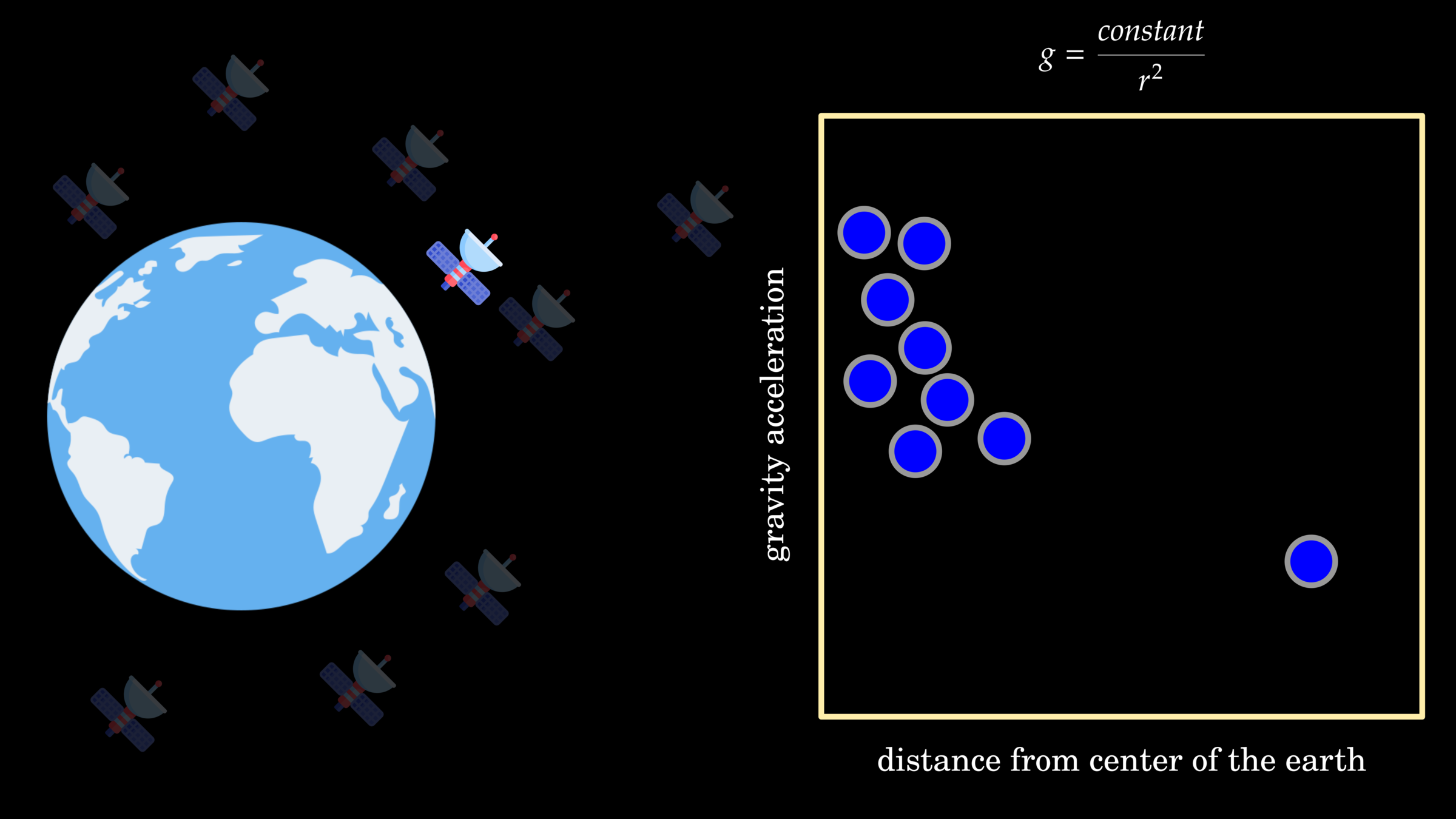
The theory-driven approach is rooted in the principles of established scientific theories and concepts. It involves forming hypotheses based on these theories and then designing experiments or studies to test these hypotheses. For example, Newton's laws of motion were conceptualized based on theoretical reasoning and then validated through numerous experimental tests.

The strength of a theory-driven approach lies in its basis in established scientific principles, giving the results credibility and allowing them to be integrated into broader theoretical frameworks. Its limitations, however, may become apparent when dealing with highly complex systems where the theory may not be comprehensive or completely accurate.
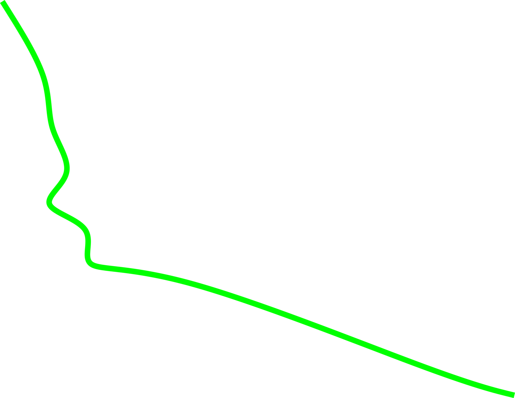
The data-driven approach shines in situations where data collection is significantly more cost-effective than physical experimentation or direct observation. In this approach, massive amounts of data are gathered and analyzed with the help of algorithms, which can identify patterns and correlations without the need for pre-existing theories or hypotheses.

For example, predicting crop types based on satellite imagery using machine learning algorithms can be much more cost-effective than physically inspecting each field. These algorithms can make sense of large amounts of data, identifying patterns that might not be visible to the human eye, and making accurate predictions based on these patterns.

The data-driven approach excels in its ability to handle vast quantities of data and uncover unexpected patterns, providing novel insights. However, it might not always provide the underlying causal relationships or be as easily interpretable, as it's primarily focused on correlations in the data.
Theory-Driven Approach
Data-Driven Approach
The commonality between theory- and data-driven is recognizing the phenomena patterns to create an equation. However, data-driven needs data to create a model, and theory is anchored in observation and deductive reasons.
artificial intelligence
data science
deep learning
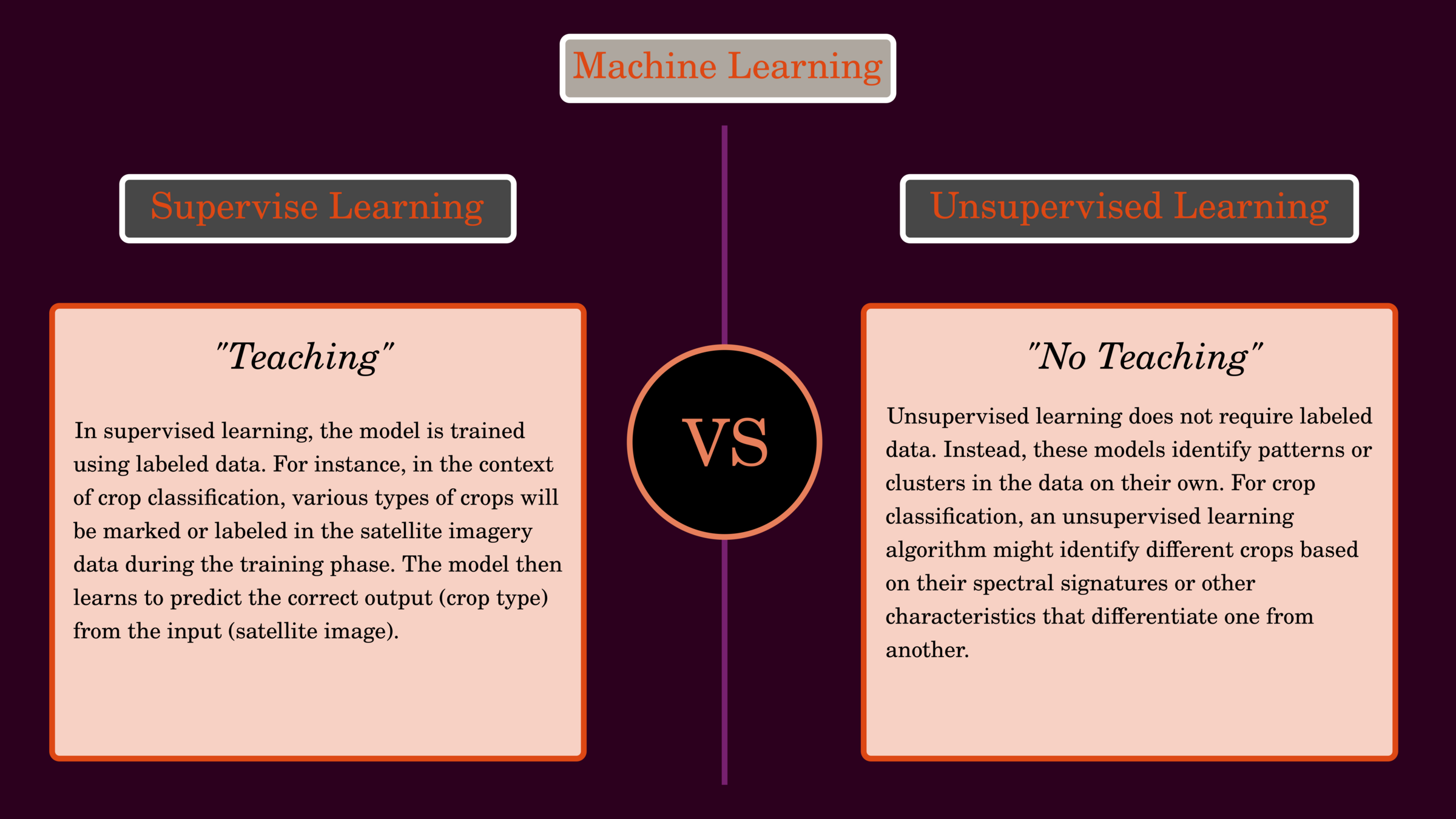
supervised learning
unsupervised learning
geometric deep
learning
machine learning
data analytics
big data
1950s
1960s
1970s
1980s
1990s
2000s
2010s
The term "Artificial Intelligence" is coined by John McCarthy at the Dartmouth Conference.
The "nearest neighbor" rule was formulated, a foundational concept for what would become known as the field of pattern recognition in machine learning.
The concept of backpropagation begins to be explored, but it doesn't get much attention until the mid-1980s.
Yann LeCun developed the LeNet-1, one of the earliest convolutional neural networks, which was used to recognize handwritten numbers on cheques.
Support Vector Machines (SVMs) are developed, providing a robust approach for supervised learning tasks.
The term "Deep Learning" is introduced to the machine learning community by Hinton and Salakhutdinov.
AlexNet, a convolutional neural network designed by Krizhevsky, Sutskever, and Hinton, achieves a top-5 error rate of 15.3% in the ImageNet 2012 challenge, significantly better than previous designs, bringing convolutional neural networks and deep learning to the forefront.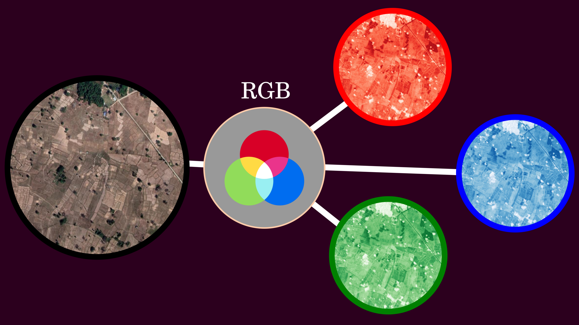
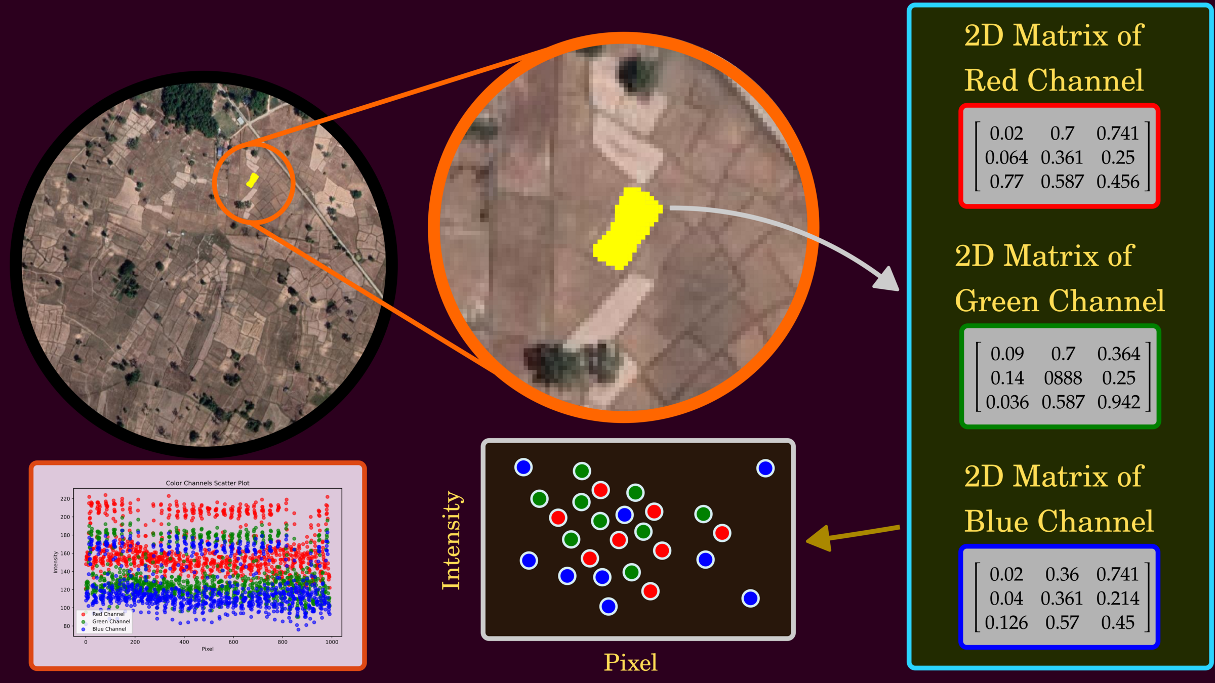
Understanding Data
One of the most standard display colors in terms of the pixel is RGB, and this composition provides natural blend color look.
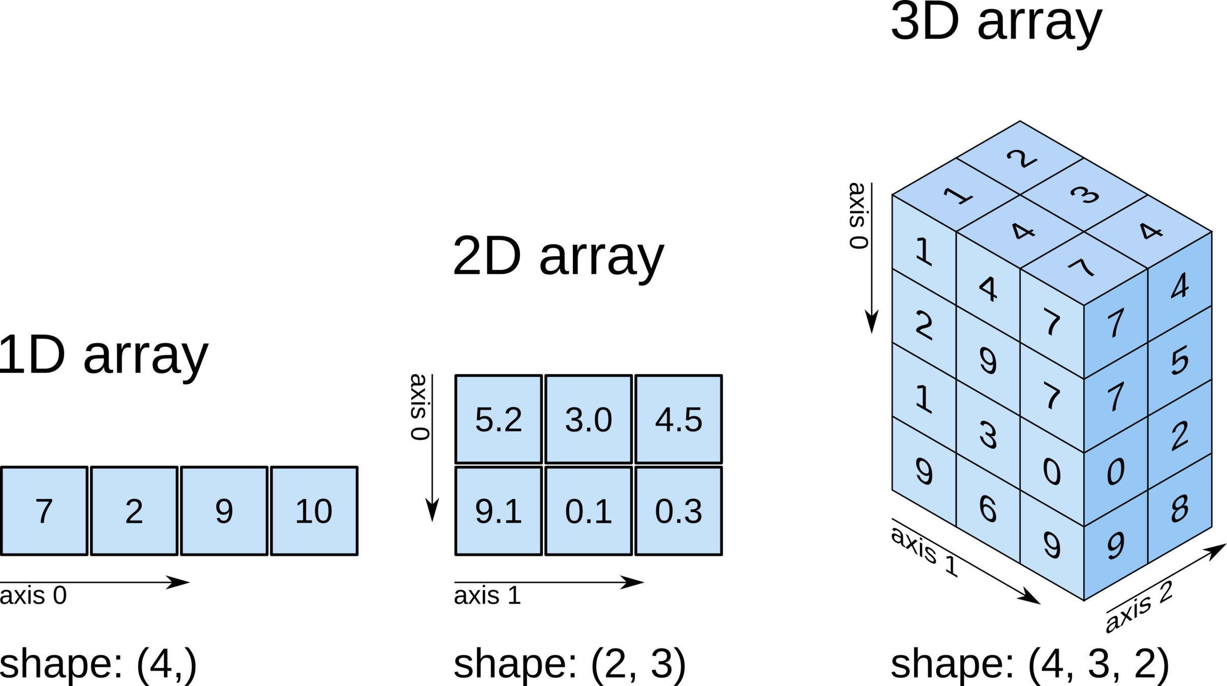
Scalar, Vector, and Tensor
Understanding the Data
Basic Data Clustering
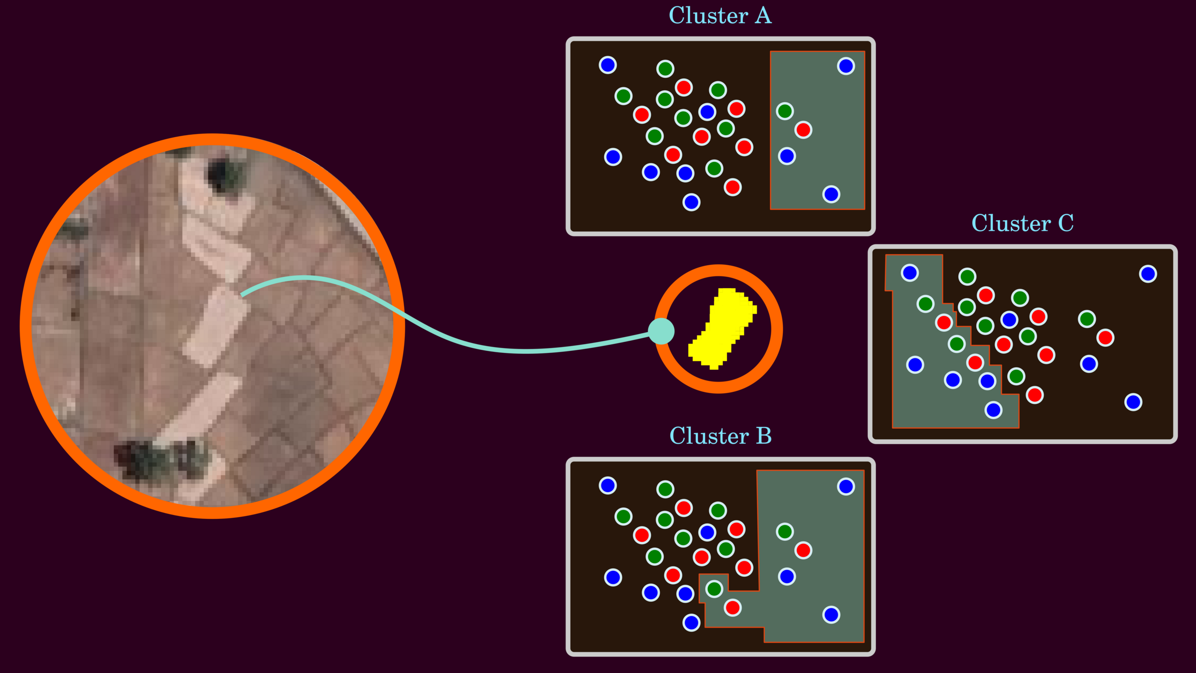
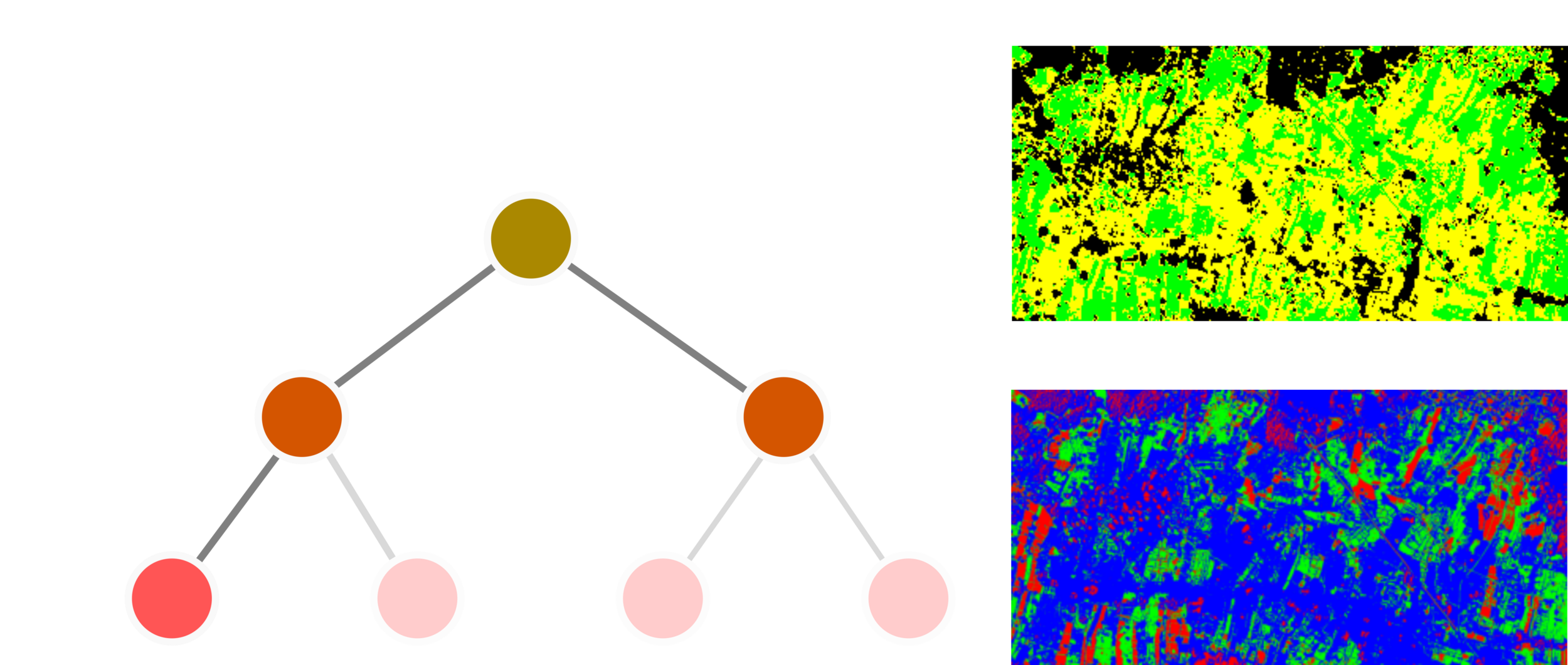
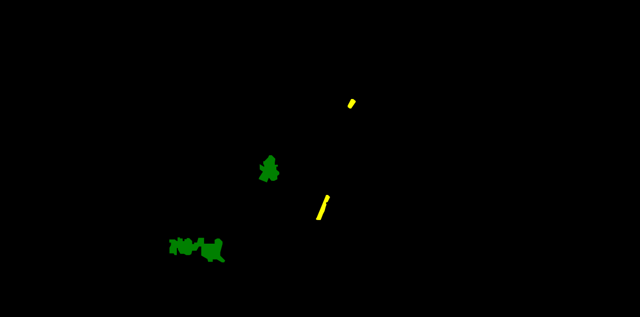
The clustering data aims to cluster one paddy rice from the image, and three scenarios could segment it correctly.
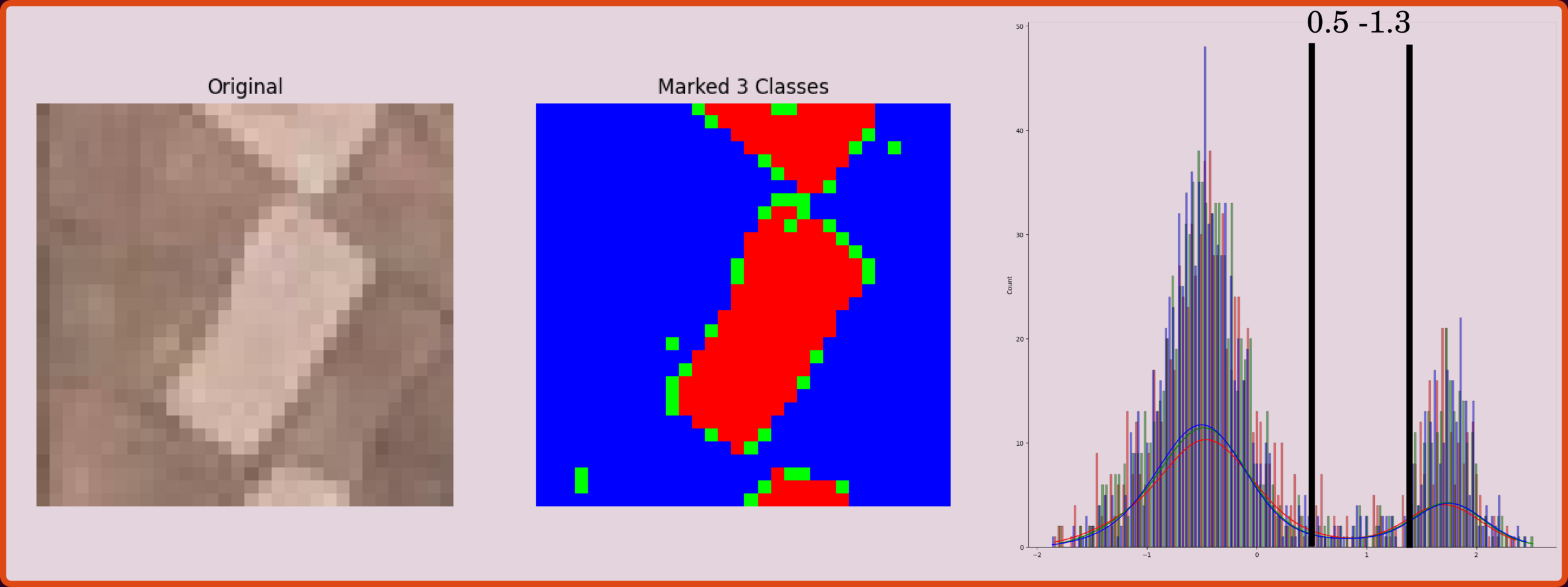
Basic Data Clustering: Clustering by a Value

This processing step uses a simple if-else statement to cluster the rice paddy, showing as black masks.
Cutoff >= 200
Data in Normal Distribution
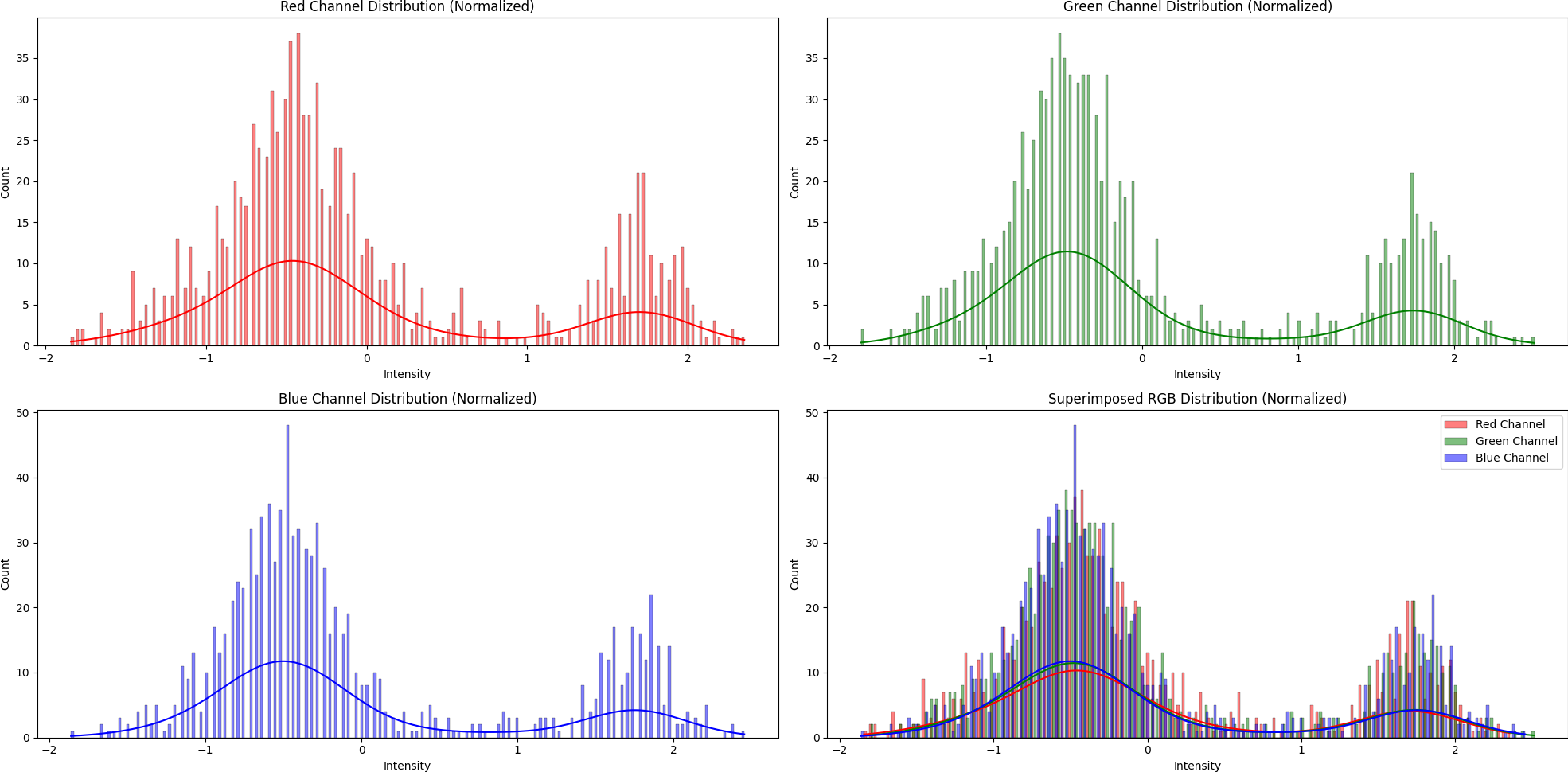
Clustering Data: Threshold-Based Method
Based on intensity distribution, we can design various cutoffs for simple clustering data. This traditional technique is simple but prone to error when applied across domains or changing a dataset.
Supervised Learning: Decision Tree
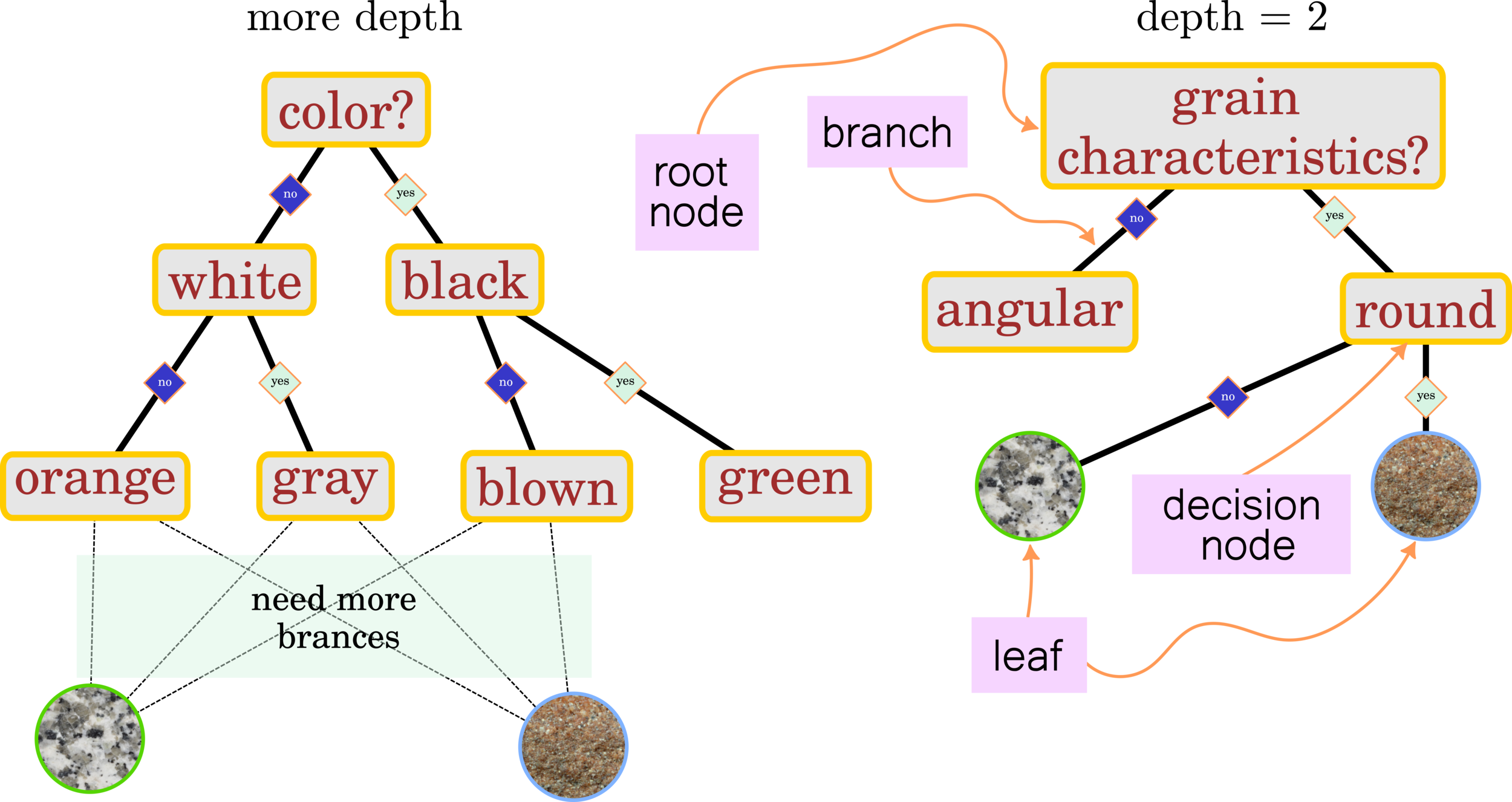
One of the most simple techniques of classtering data is to use an if-else statement to create generalized rules to group the scattering data. The previous work uses a simple cutoff of 0.5-1.3 to cluster the rice paddies. However, when the data cover a large area, they need to increase the tree depth (creating more conditions).
Unsupervised Learning: K-means
input data
locate centroids
measure distances
relocate centroids
distance equal threshold
end
yes
no


find the shortest paths between each data point and centroid.
yes/no condition, the program will end if the shortest distances between centroids and data points equal the threshold (near 0)

done! good job
CH 3: Machine Learning Pipeline
Pipeline
-
Downloading satellite imagery
-
Removing high could cover images
-
Compositing bands into RGB with proper clip value
-
Converting TIFF to PNG
-
Normalizing data
-
Removing outliers
-
Labeling classes
-
Augmenting data
XGBoost
Hyperparameter-tuning
Confusion matrix:
-
F1-score
-
Precision
-
Recall
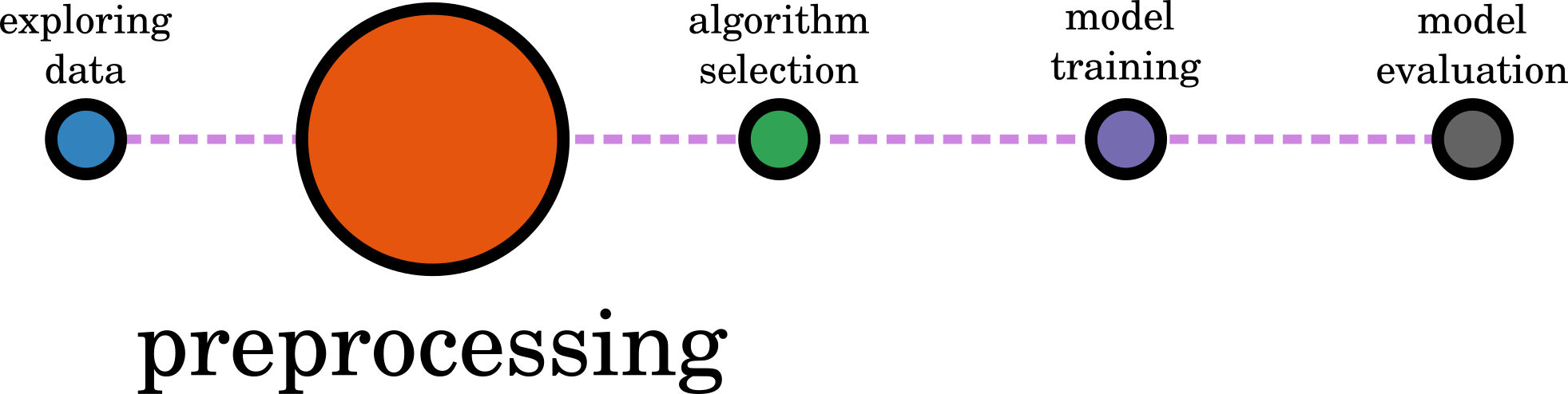
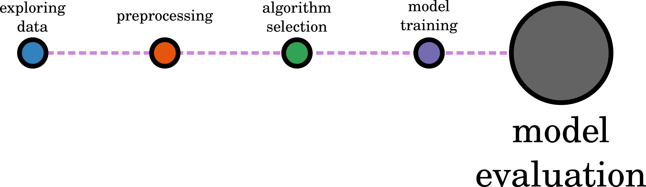
QC Data
Processing
Data
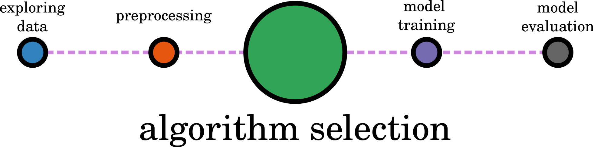
Algorithm Selection
Model
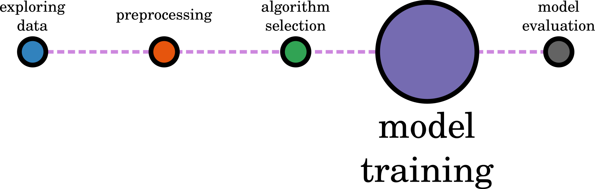
Traning
Model
Evaluation
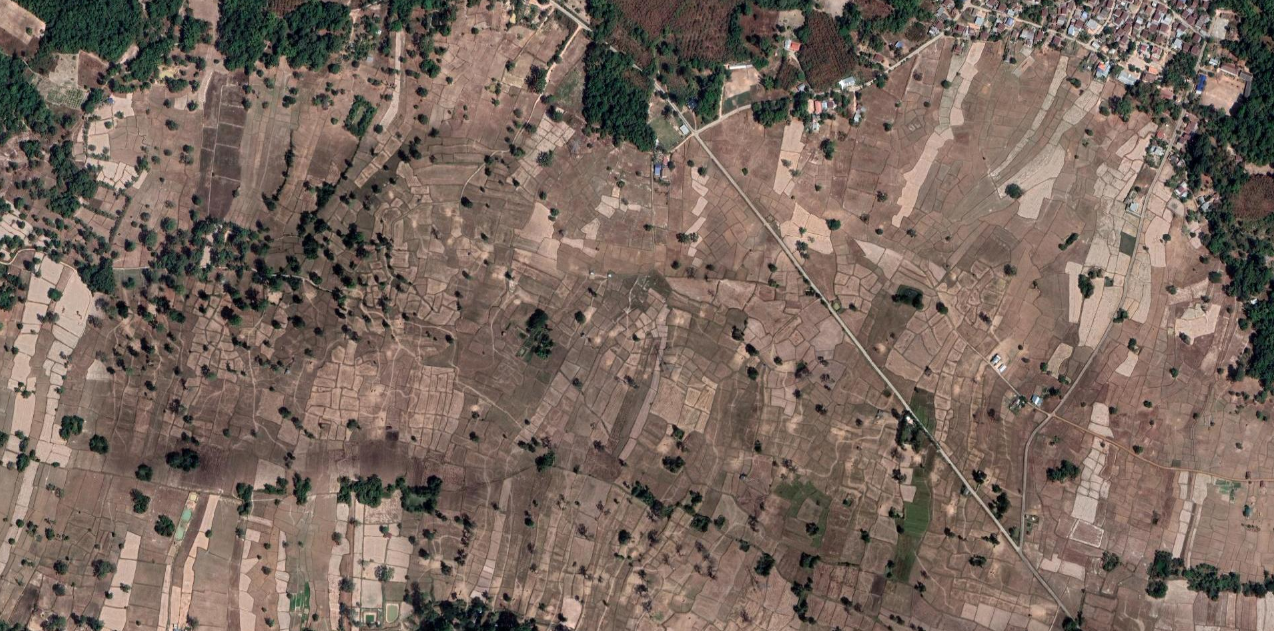
Downloading High-Resolution Satellite Imagery
Normalization

Often time that input data varies in range, so comparing multiple datasets is more efficient when they share consistent lengths.
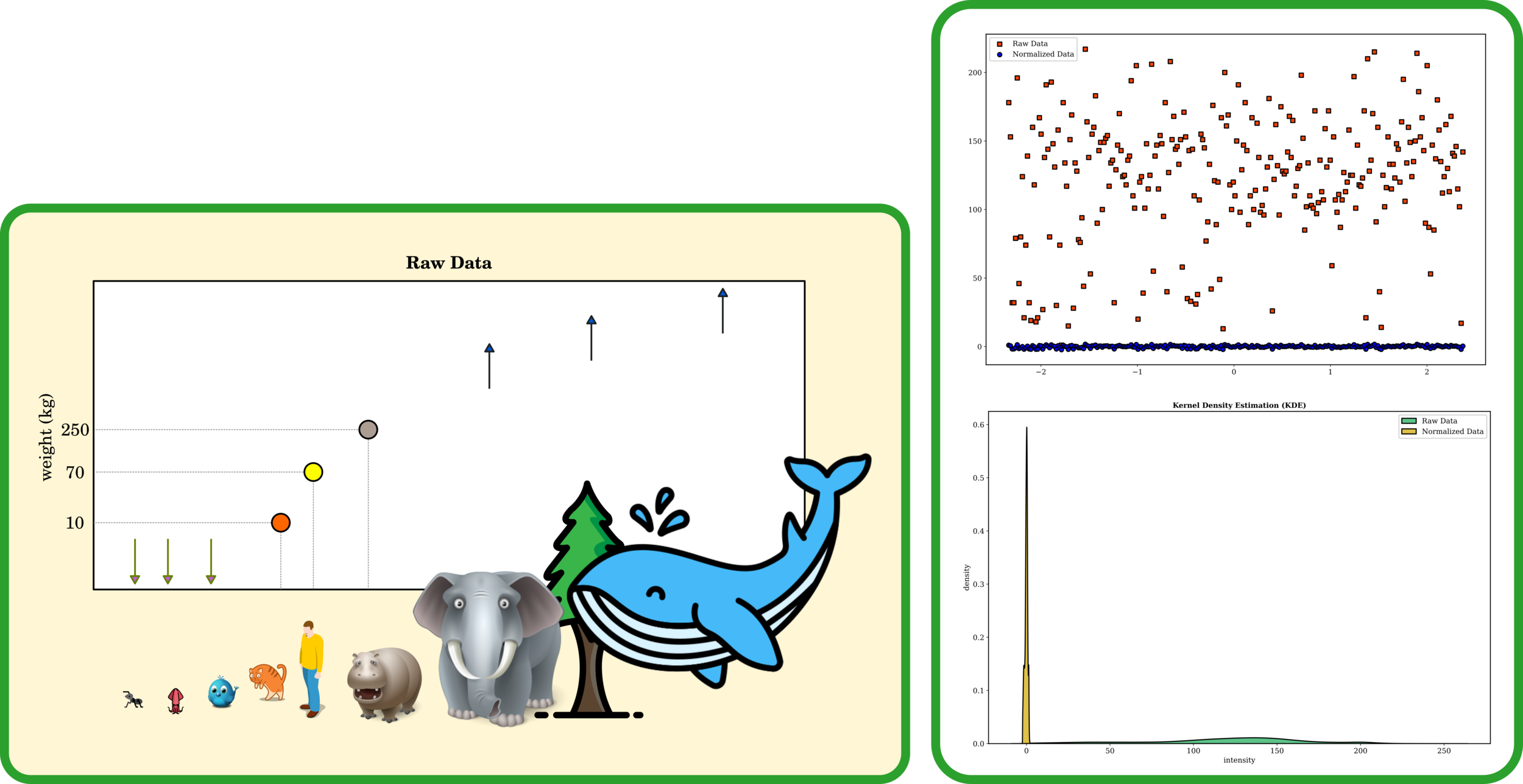
Outlier Remover
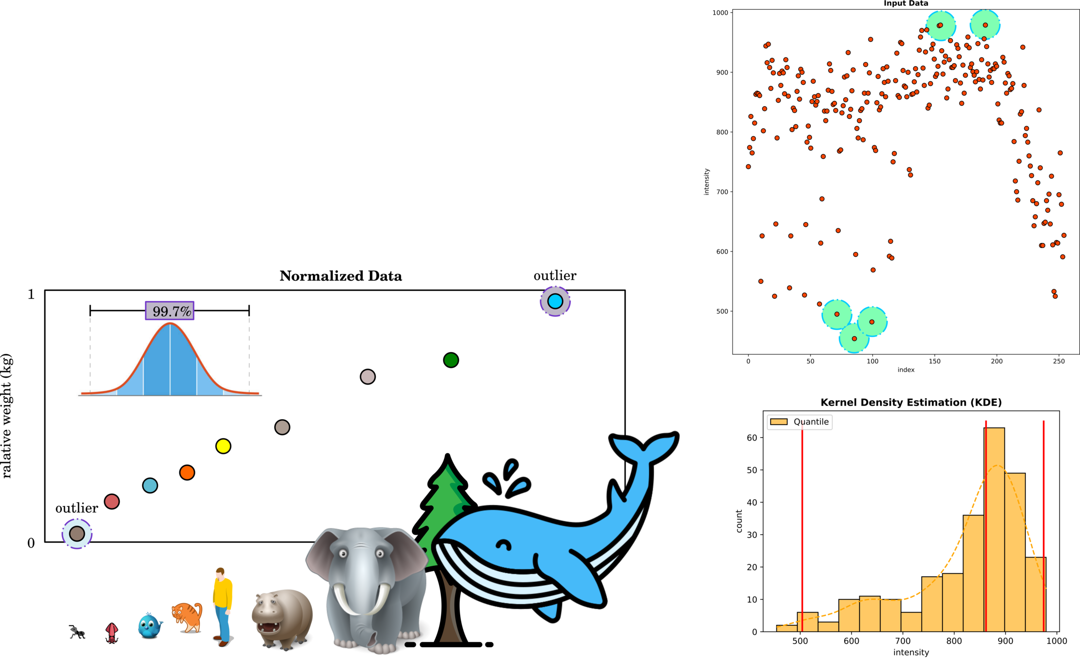
Outliers are data points that isolate from the density, and these points might lower the model accuracy.
Data Labeling
Our goal for this project is to develop a machine learning model that accurately identifies rice paddies in satellite imagery. We'll use the XGBoost algorithm, a supervised learning technique based on decision trees. To achieve this, we'll label different sections of the image to train the model. This training process will teach the model to correctly categorize each segment of the image, determining whether it represents a rice paddy or not.
Label
Algorithm Selection

Model Training
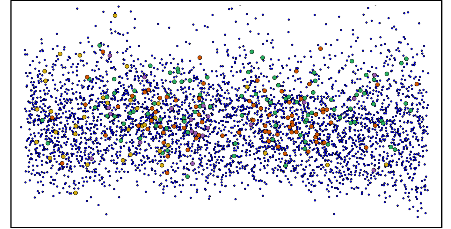
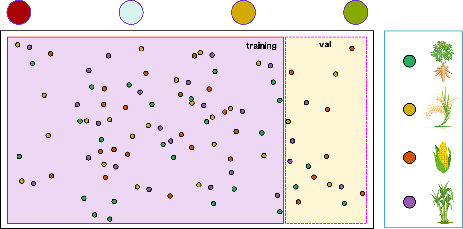
ML is a data-driven approach requiring big data to construct an algorithm, utilizing some parts of input data for training and validation, and this technique calls splitting data.

So which part of the data should be used for training and validation then?
Some thoughts
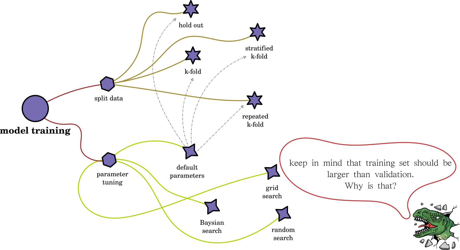
Cross-Validation
training = A+B+C+D
validation = E
test = F
click
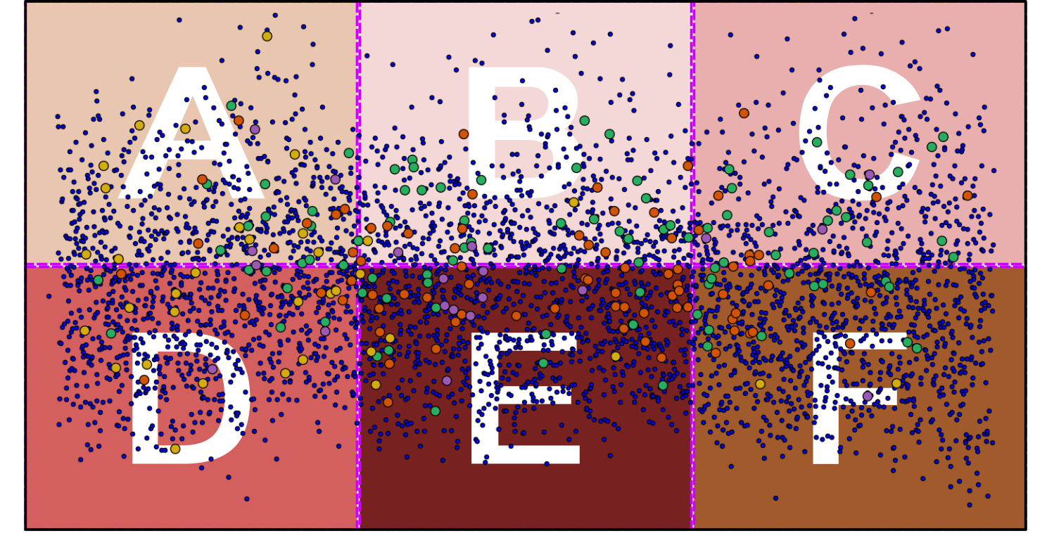
Which section of the data should utilize as
training,
val, and
test?
Or is there
a better way!
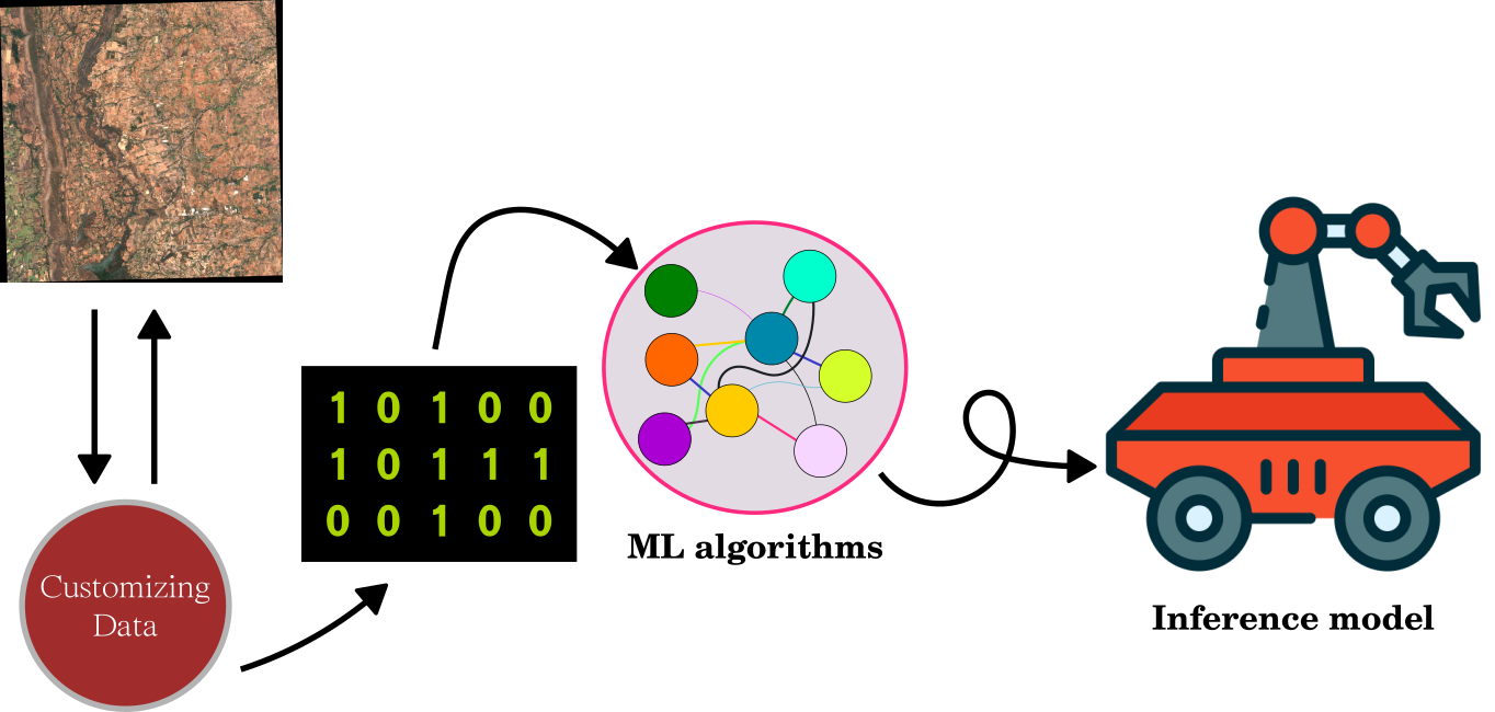
Revisit Data-Driven Approach
One customizing data or adding new data into ML will end up with different inferences.
So which input data plus preprocessing is the best?
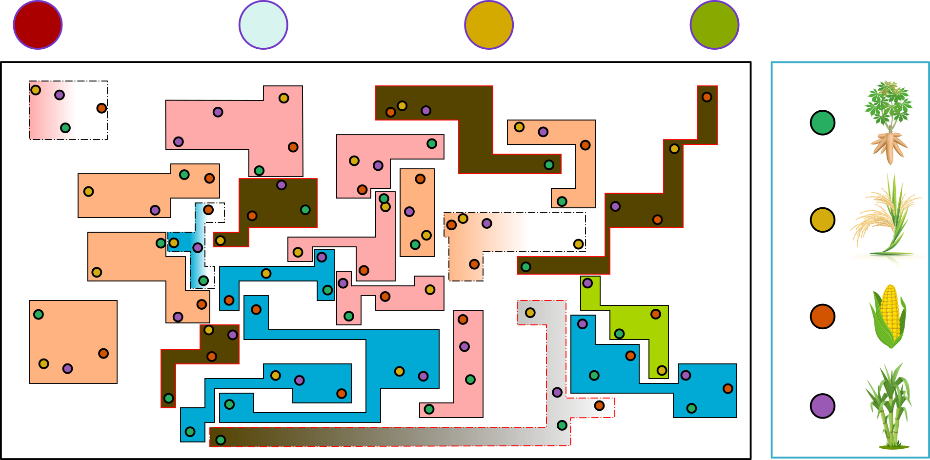
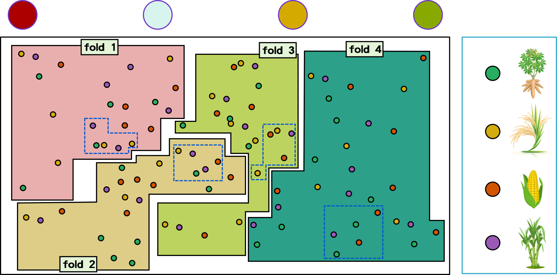
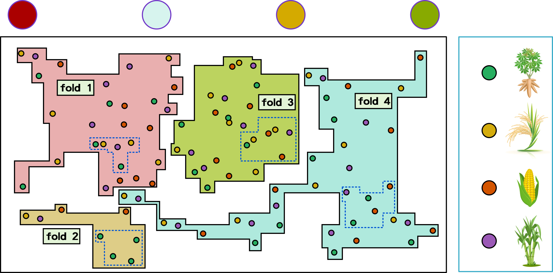
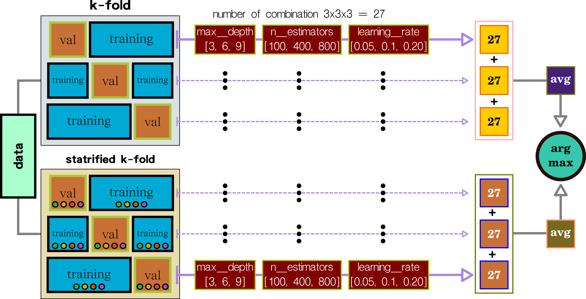
Cross-Validation Types
hold-out
fix splitting ratio
split data into a number of designed folds with constant size
k-fold
repeated k-fold
split data into a number of designed folds with various sizes
split data according to classes into a number of designed folds
stratified k-fold
Parameter Tuning + Split Data
"huge computation"
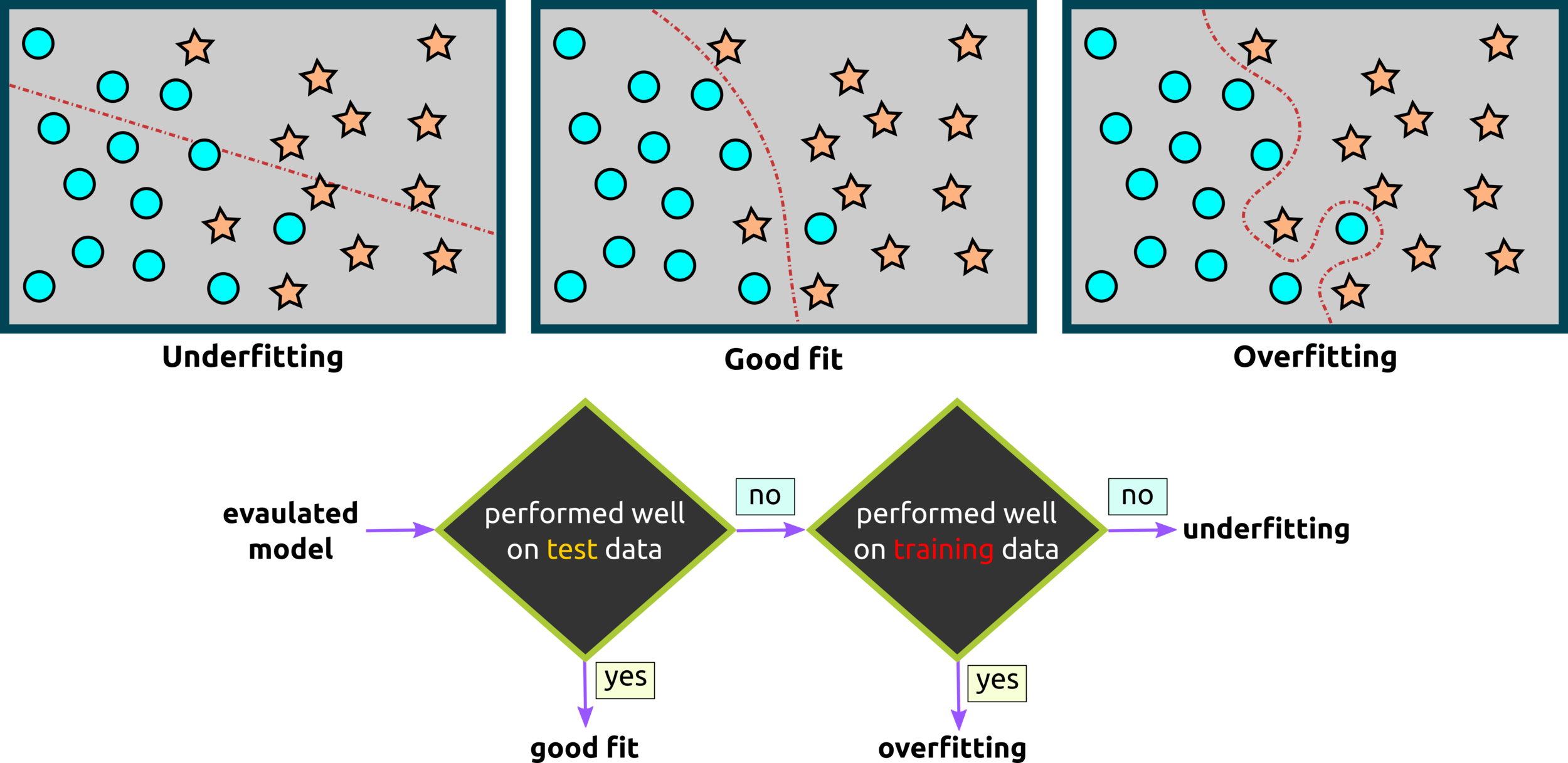
Underfitting - Good Fit - Overfitting
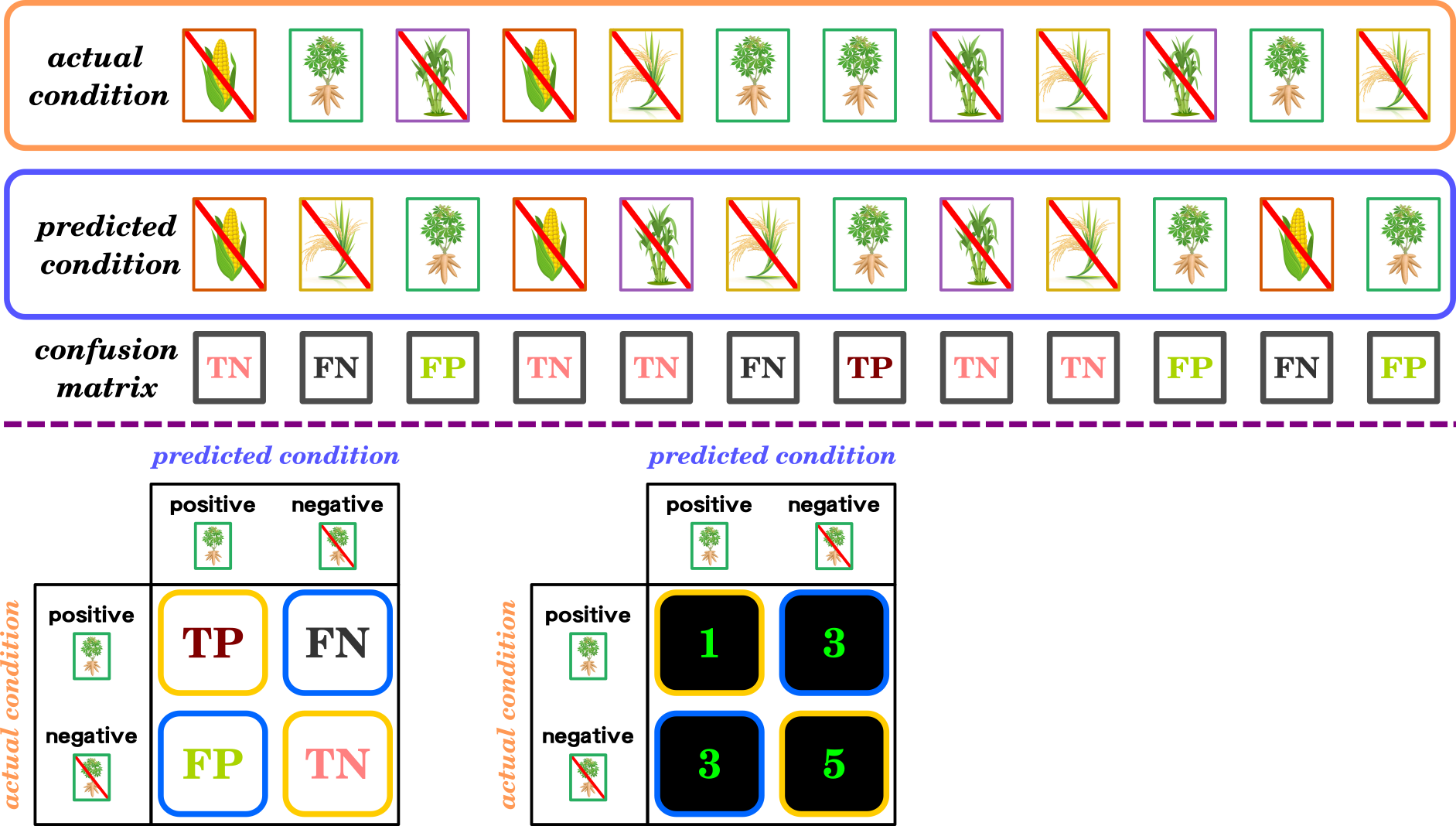
Confusion Matrix for Binary Classification
\displaystyle precision=\frac{TP}{TP+FP}
\displaystyle recall=\frac{TP}{TP+FN}
\displaystyle F-1\ score=\frac{2TP}{2TP+FP+FN}
Hyperparameter Tuning: Grid Search, Random Search, and Bayesian
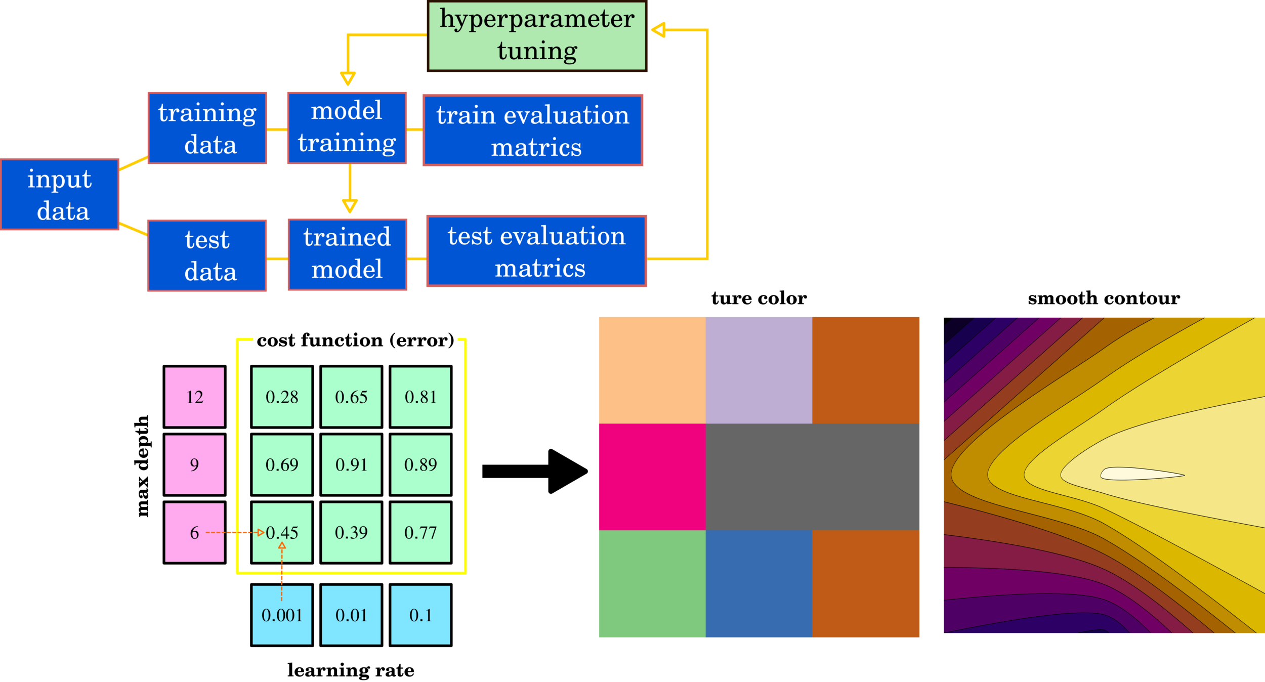
XGBOOST contains several parameters that require trial-out and error to find the best parameter set. The most straightforward technique is grid search which tries all parameters. The random search uses an intelligent method to select a potential test set—both methods consume a lot of trail-out and error. The current method is Bayesian optimization, which can automatically narrow the optimal range of the test set.
best window
CH 4: Basic Math for Machine Learning
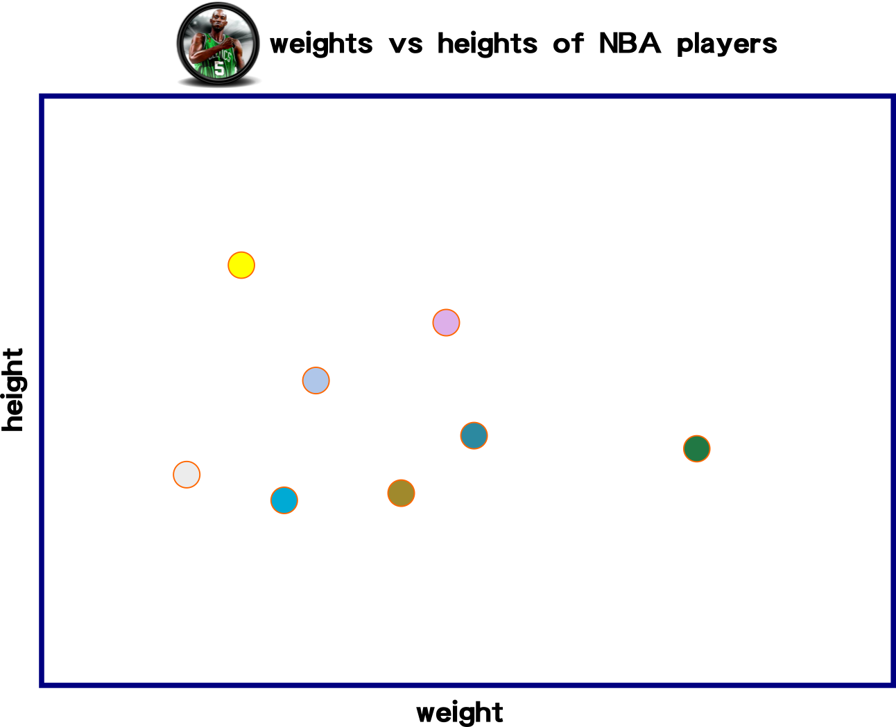
Big Picture: Linear Regression
input
data
iteration
2
iteration
1
iteration
k

The idea of the linear function is to create a function that can predict forthcoming input data. This slide demonstrates three linear functions for measuring the distance among data points and the linear functions.
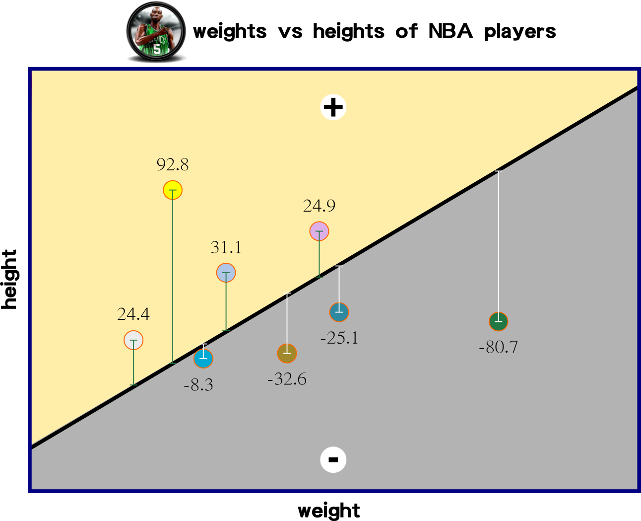
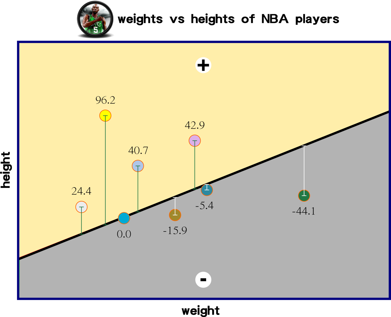
Which iterated function has the lowest sum of values?
input
data
iteration
2
iteration
1
iteration
k
the smallest errors are
the best regression
...
how many iteration then that is close to 0?
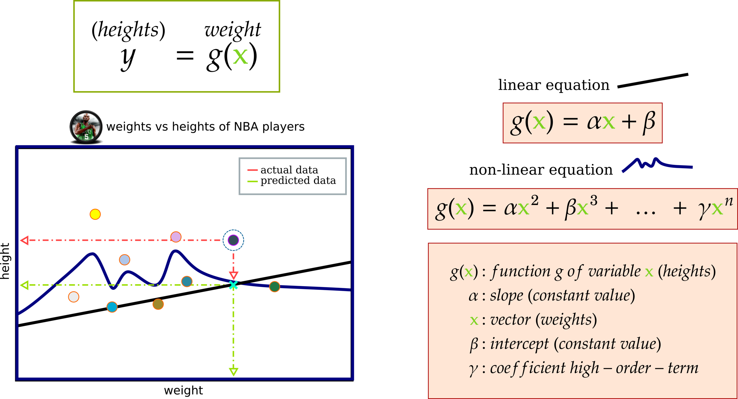
Big Picture: Non-Linear Regression
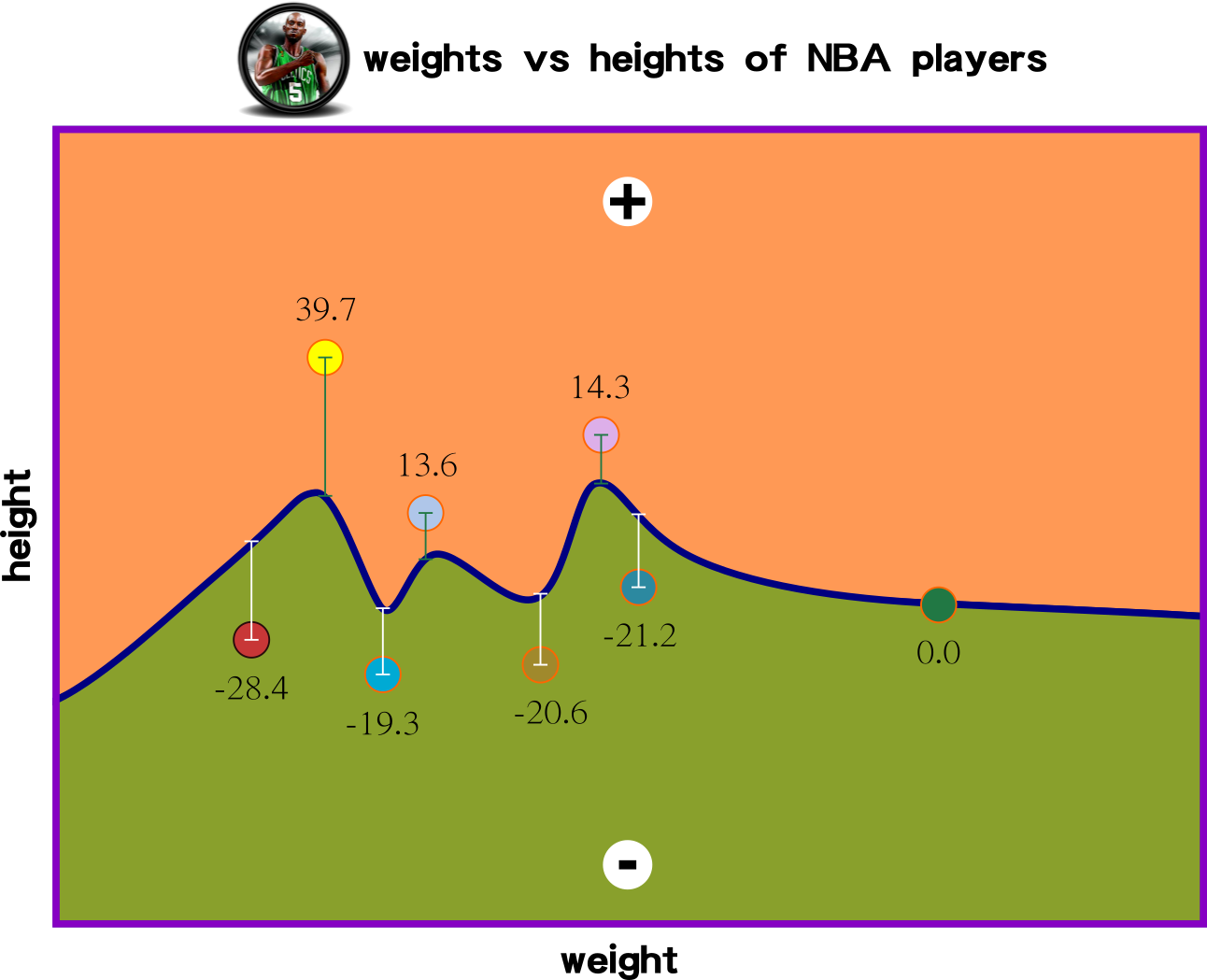
Cost Function: Measuring Model Performance
Function g(x) has a relationship with variable y. This affinity means g(x) might contain several terms to predict the behavior of variable y.
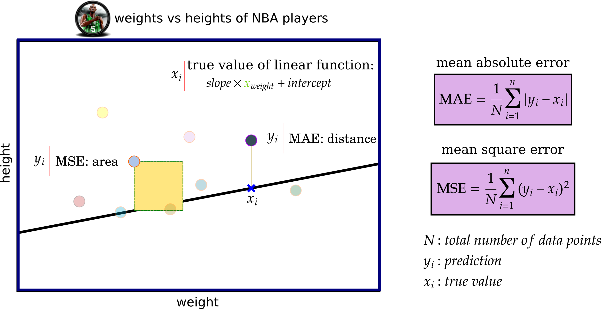
Cost Functions: MAE and MSE
Cost Function Mapping Errors


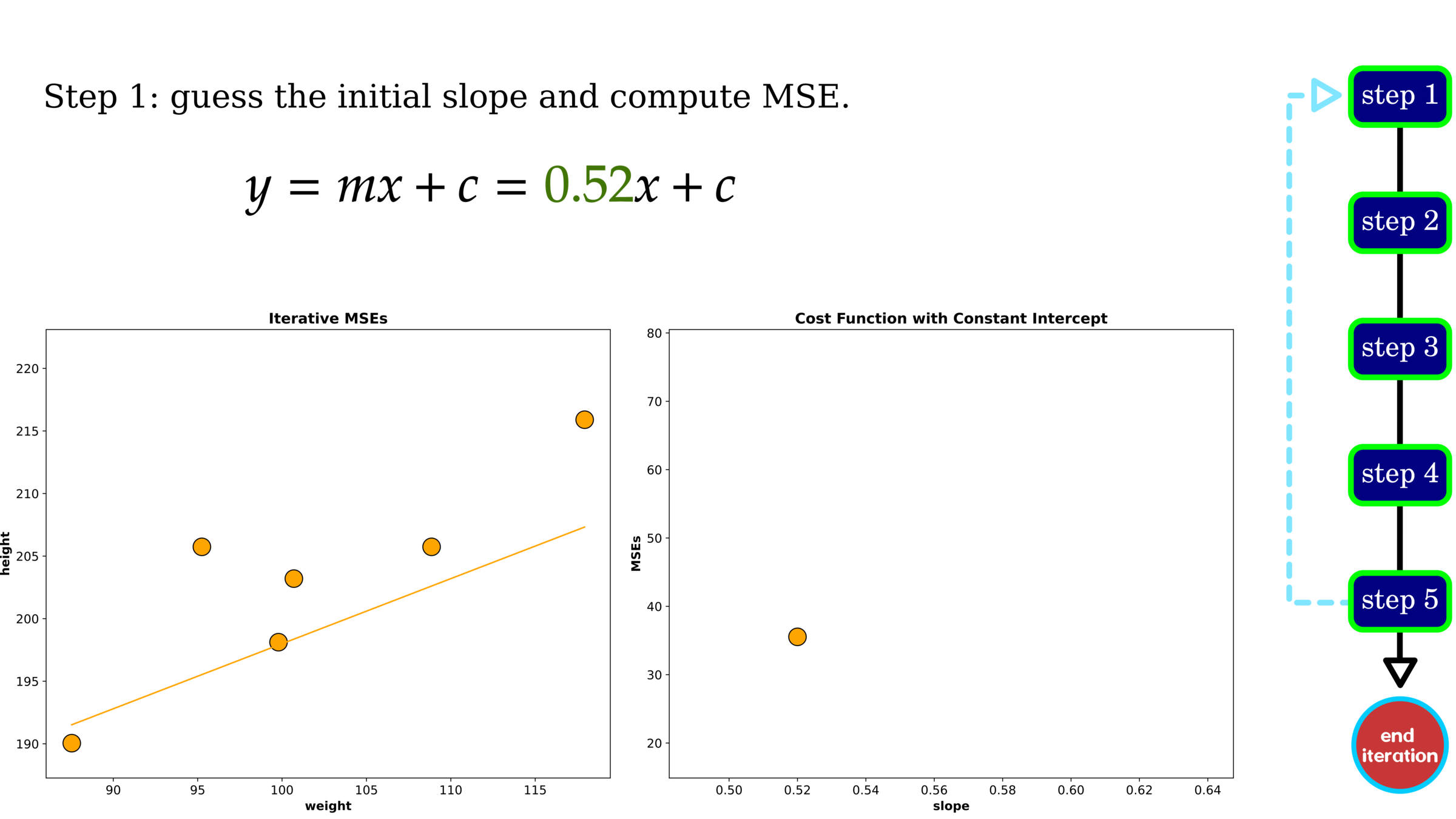
Rather than trying one pair of slope and intercept, we tested 400 values for each parameter, yielding the result on LHS. On RHS is an example of a selected pair of slope and intercept.
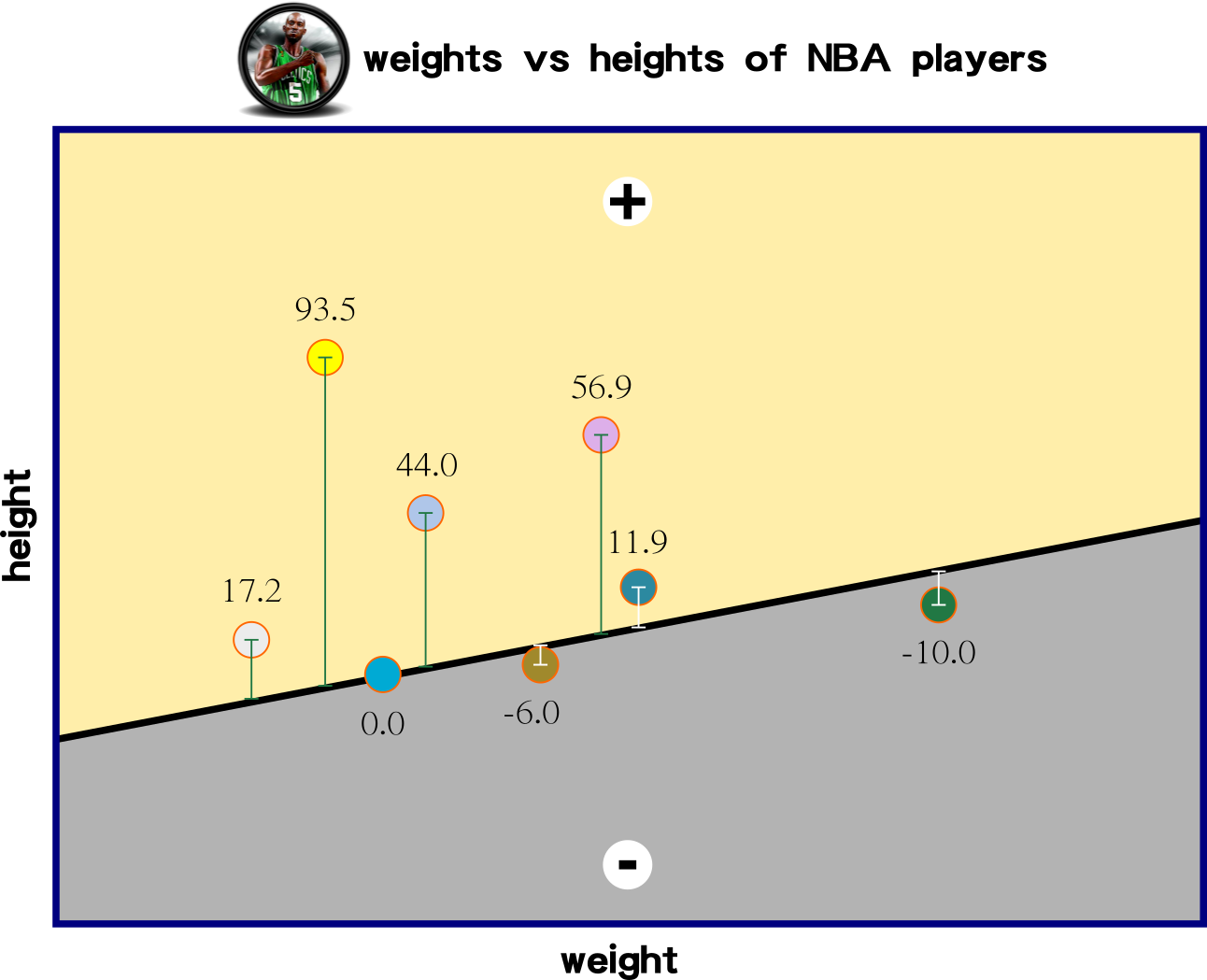
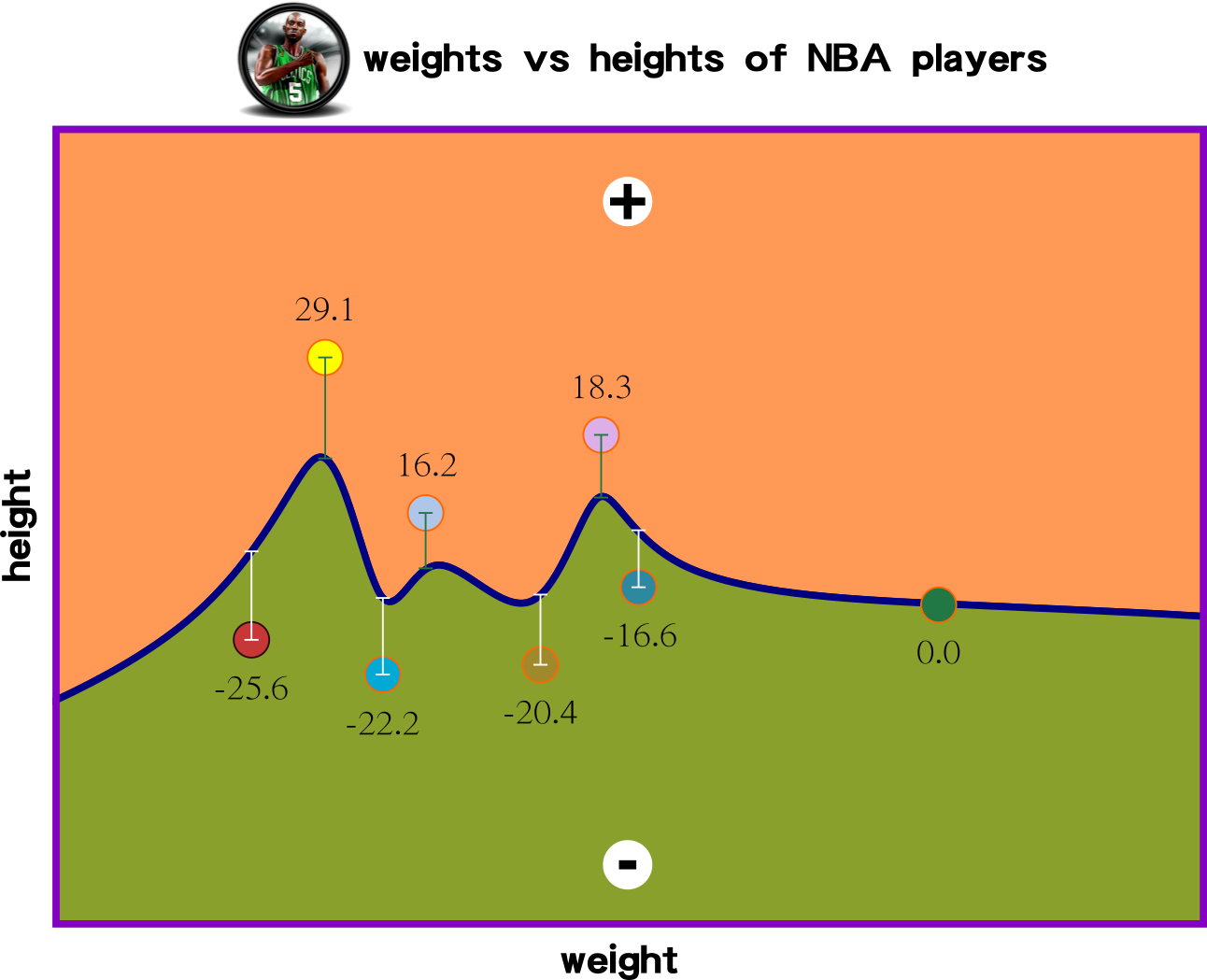
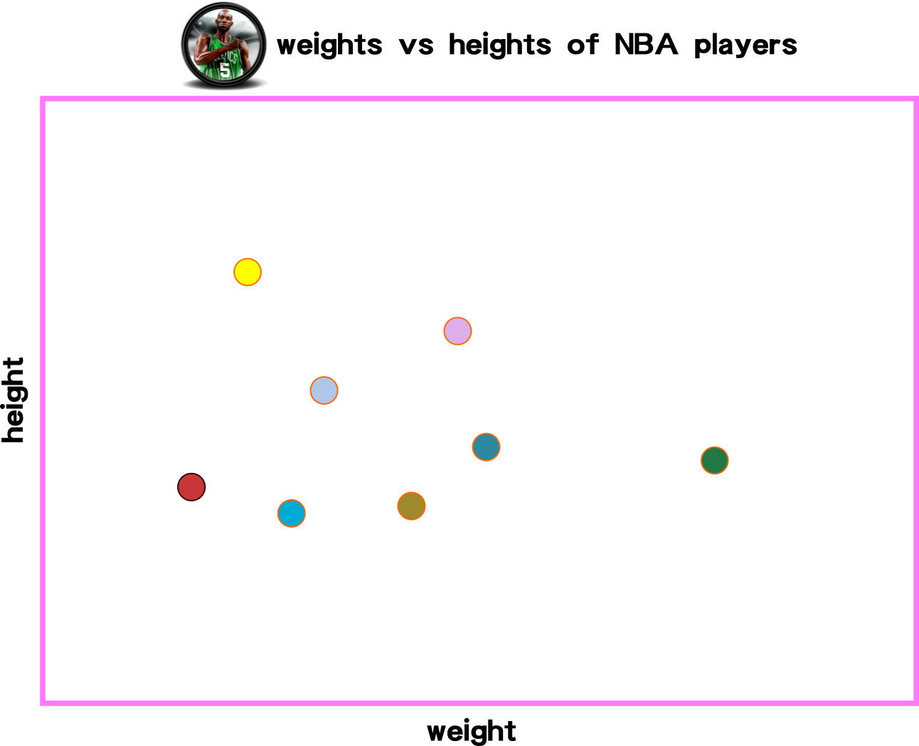
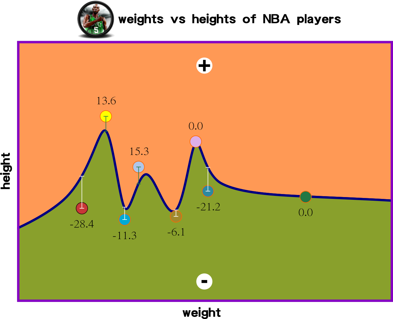
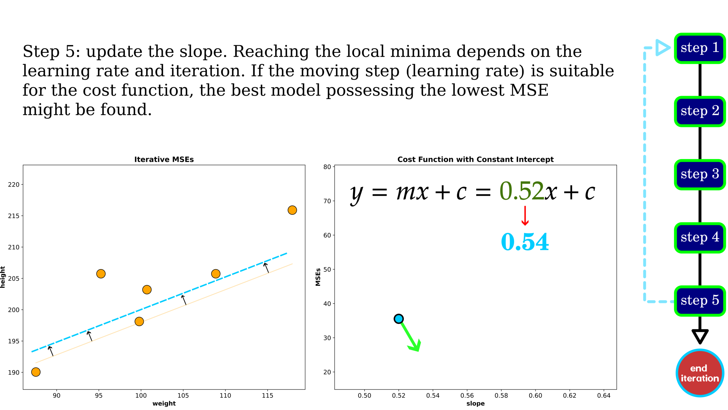
Optimization: Gradient Descent
Optimization: Gradient Descent
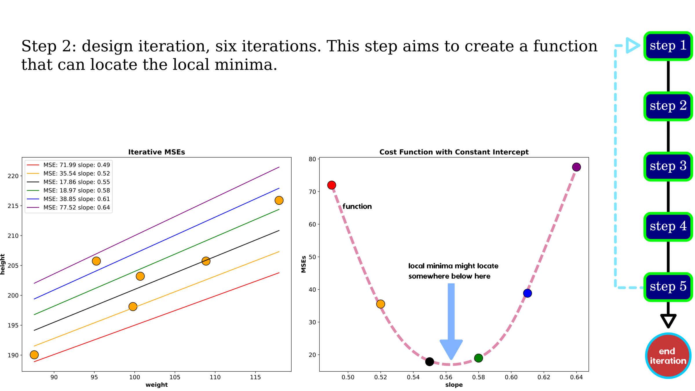
Optimization: Gradient Descent
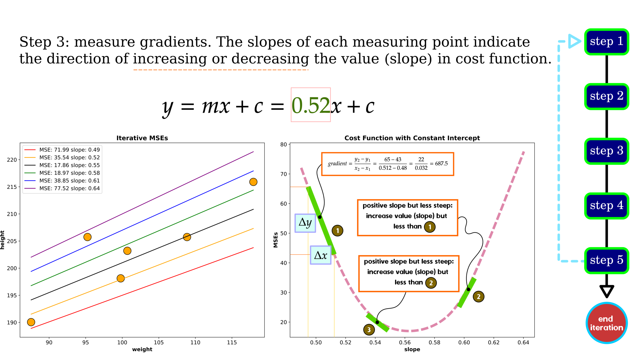
Optimization: Gradient Descent
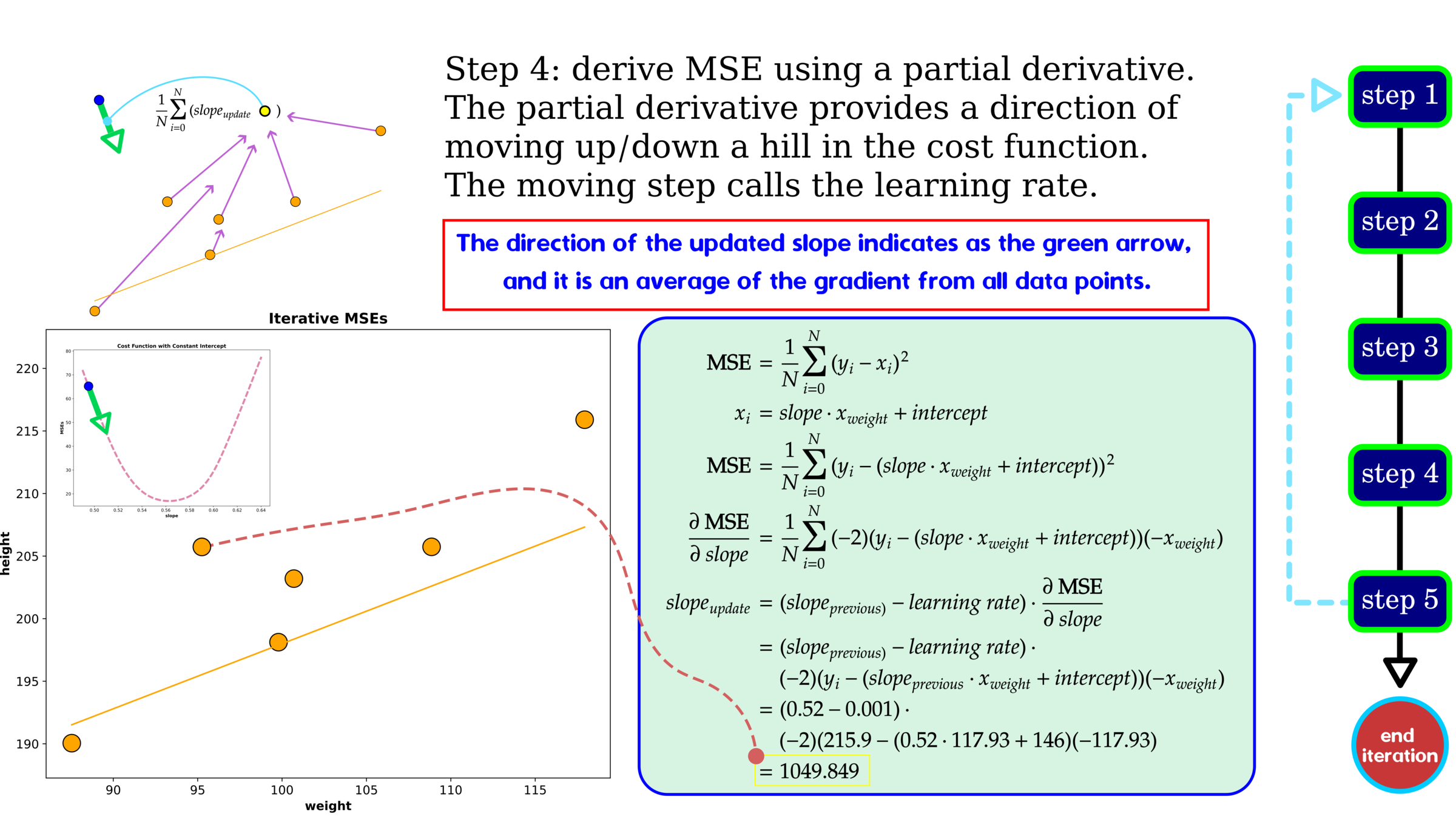
Optimization: Gradient Descent
Linear Regression Using Gradient Descent


Without hyperparameter tuning, gradient descent gives a decent MSE showing higher error than grid search. One data point on cost history indicates trail-out-and-error of tuning variables, slope and intercept. We use the cost history to search the best parameters, and in this example, after iteration 2000, the error is plateauing, indicating that the selected parameter set is found. We should stop searching at this iteration.
Decision Tree:
Rock Classification Granite vs Sandstone
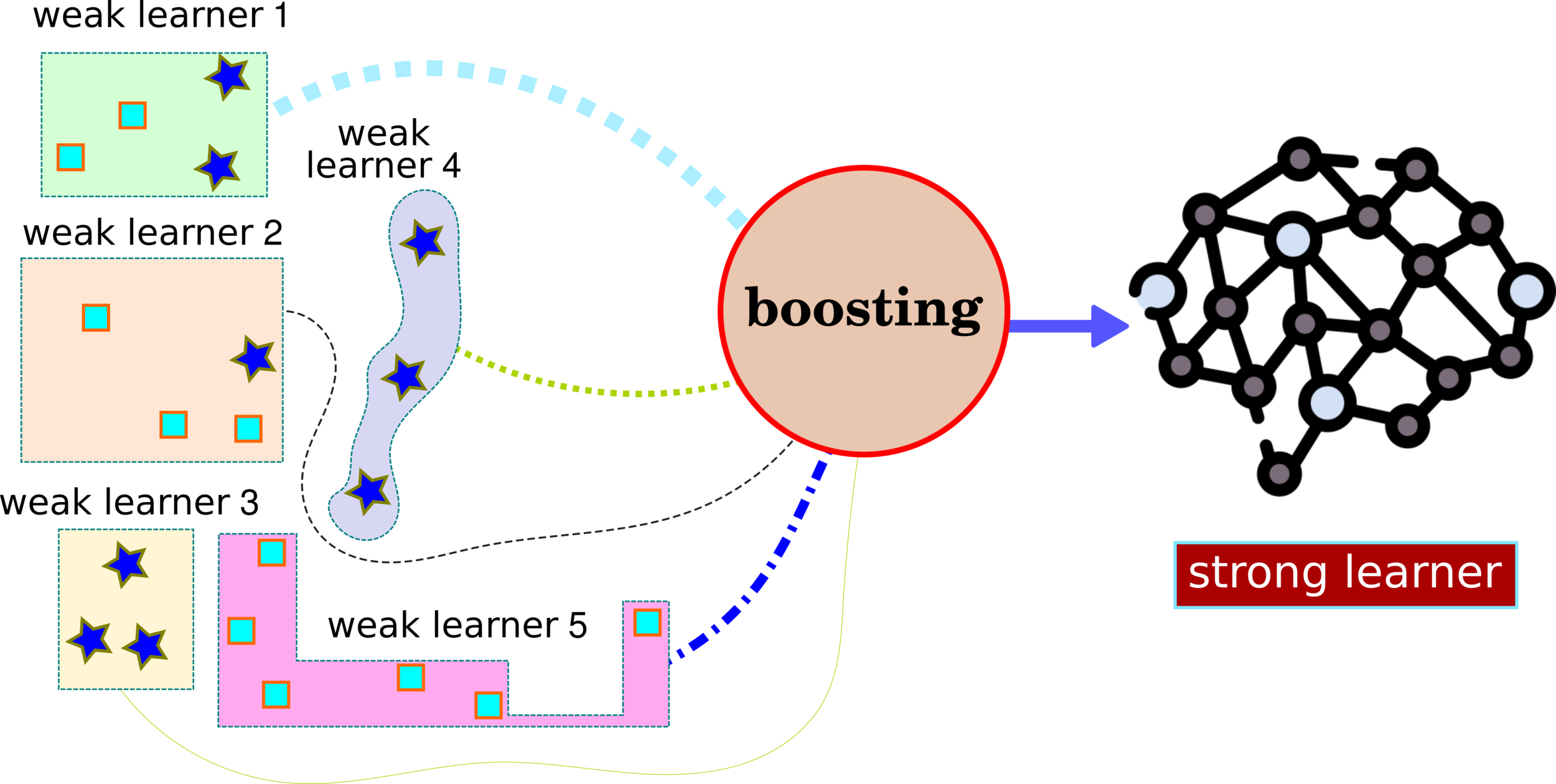
Ensemble Learning: XGBoost
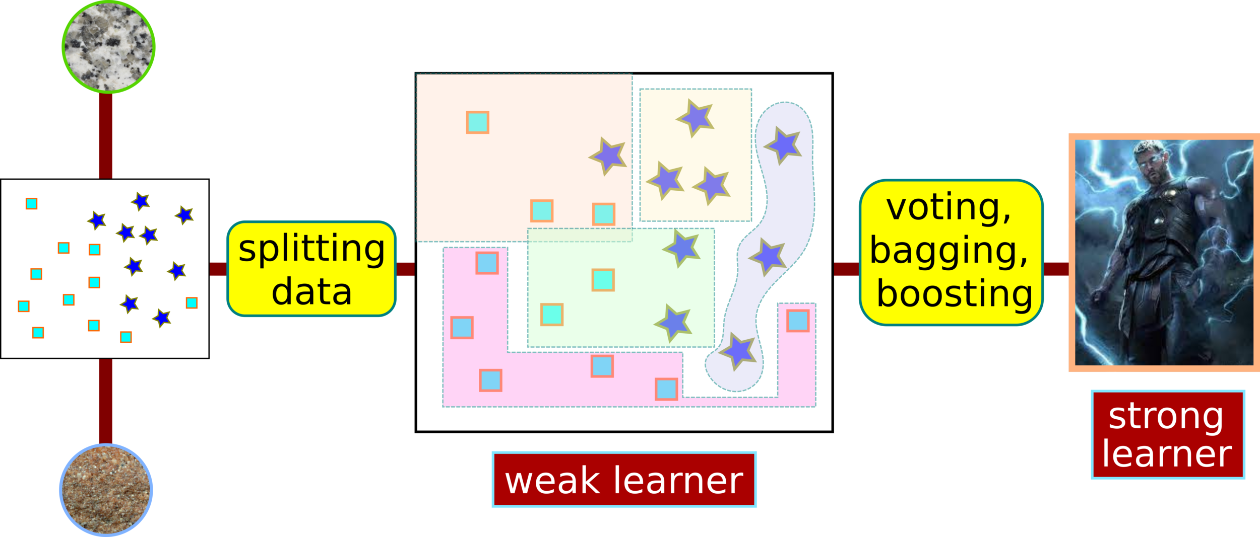
How to Split Data into Weak Learners?
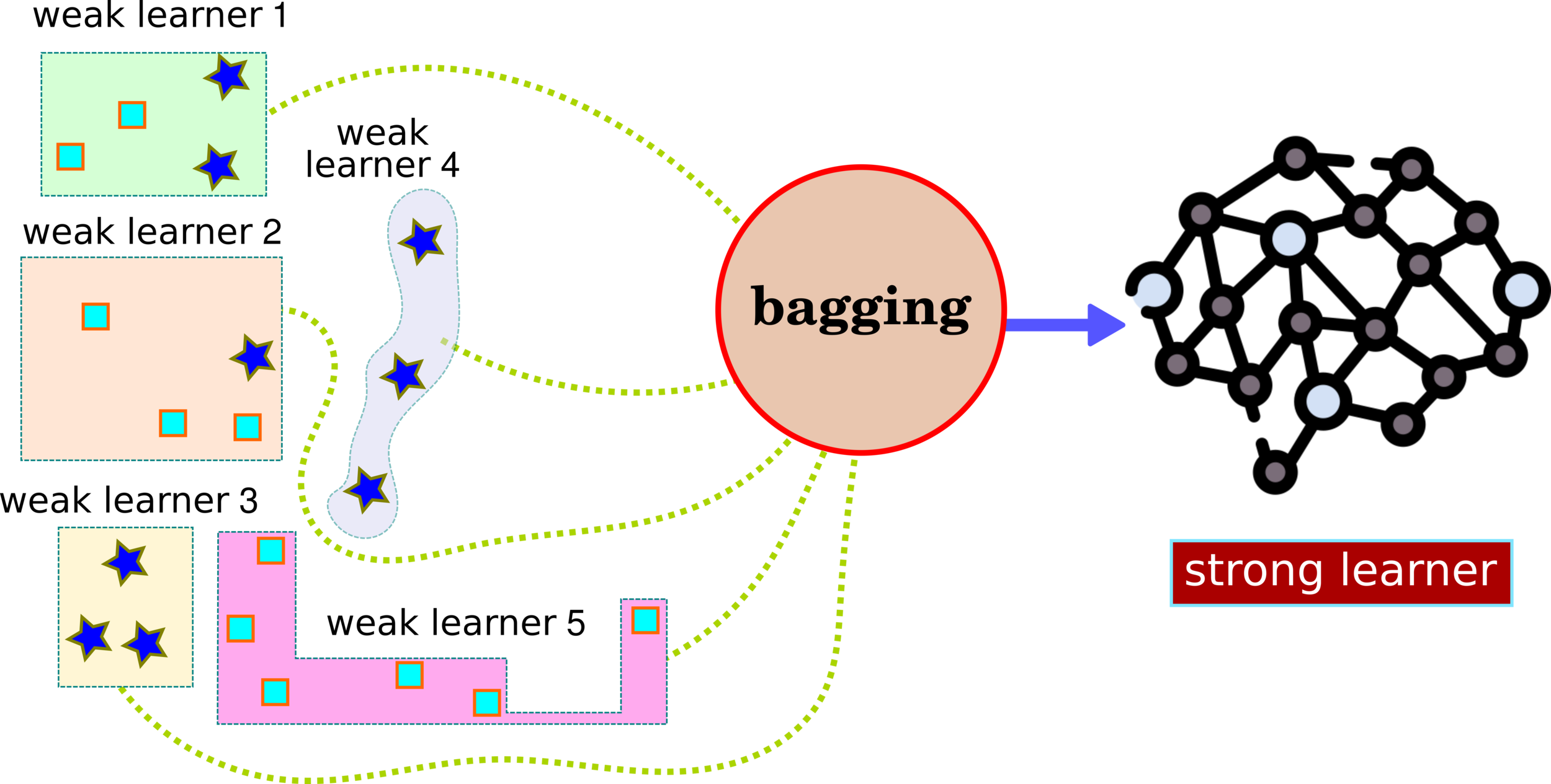
How to Split Data as a Weak Learner?
CH 5: Time Series Analysis
Forecasting
-
Predicting crop yields based on previous seasons and current growth indicators.
-
Estimating water requirements for upcoming days or weeks based on forecasted weather patterns and historical crop water usage.
Categorization of Applications in Time Series
Anomaly Detection
-
Identifying areas of a field that might be under stress due to pests, diseases, or water-logging.
-
Spotting unexpected changes in land usage or identifying fallow land.
Classification
-
Classifying types of crops in a region based on the spectral signature from satellite imagery.
-
Distinguishing between healthy and stressed plants based on their reflectance properties.
Clustering
-
Grouping similar regions or fields based on crop types, farming practices, or soil health.
-
Segmenting regions based on their response to different weather events.
Change Point Detection
-
Identifying shifts in land use, like the transition from one crop to another or from agricultural land to non-agricultural land.
-
Detecting onset of specific agricultural events like irrigation, flowering, or harvesting.
03_ML_2023
By pongthep


