Introduction to Geophysics
Fall 2022
2307358
Sep 28: backup class
Oct 19: Resistivity and GPR acquisitions
Contents
CH 0: Python Ecosystem
CH 1: Introduction
CH 2: Gravity & Magnetic
CH 3: Electrical Resistivity
CH 4: Seismic
CH 5: Ground Penetrating Radar
CH 0: Python Ecosystem
Ecosystem


Textbooks
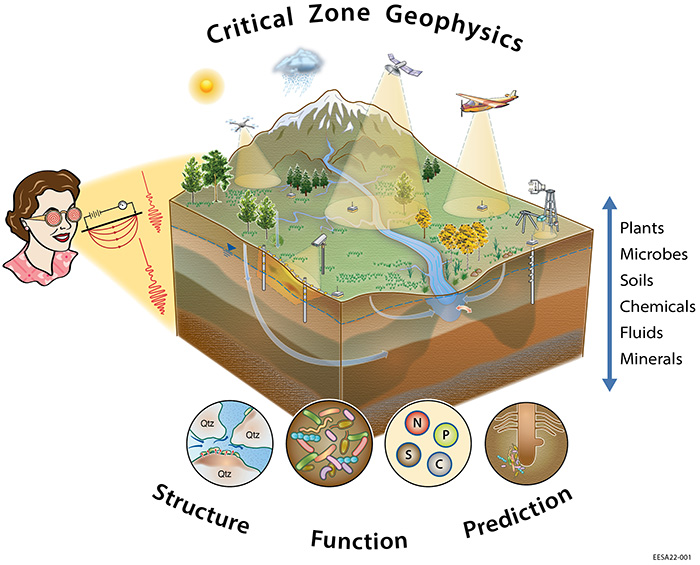
CH 1: Introduction


Geophysicists 2022
Introductory Geophysics
Introductory Geophysics

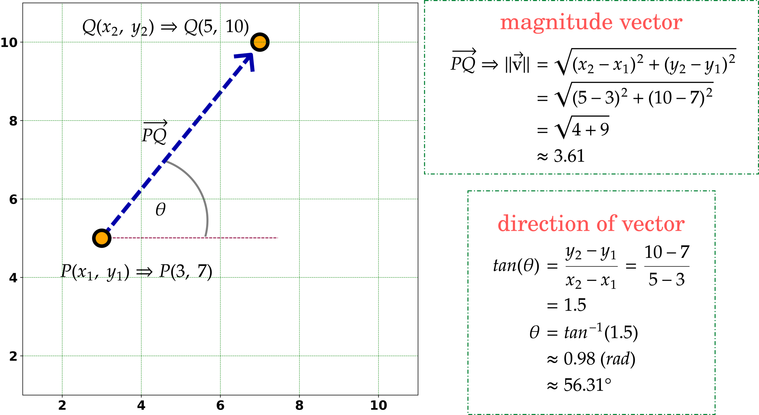
Cartesian Vectors and Functions


math notation
example
sum vector

unit vector
magnitude and direction of vectors


Vector Field: Scalar, Vector, Matrix, and Gradient
day 1
day 2
vector
field
total
field
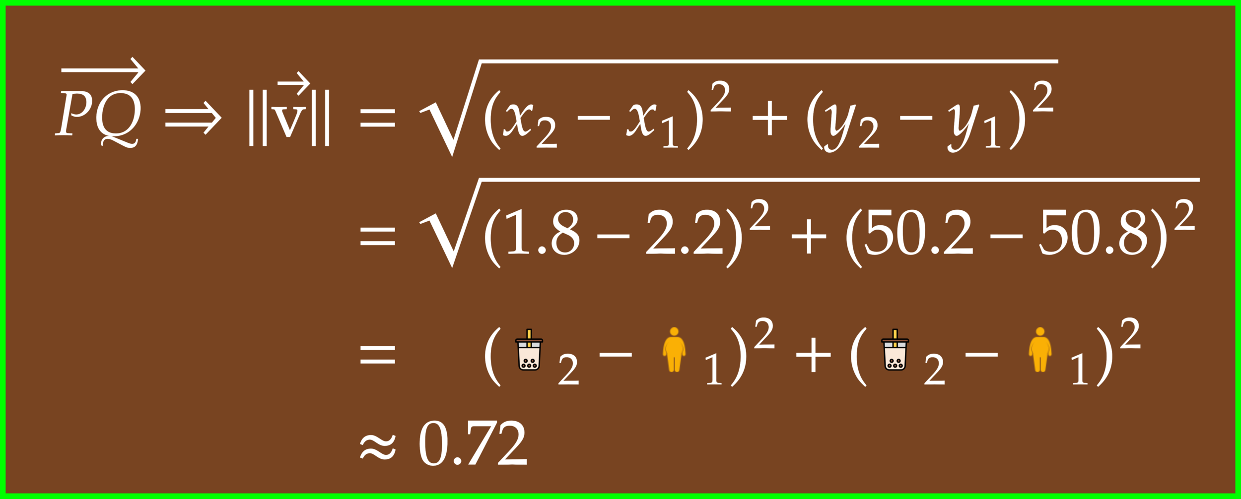
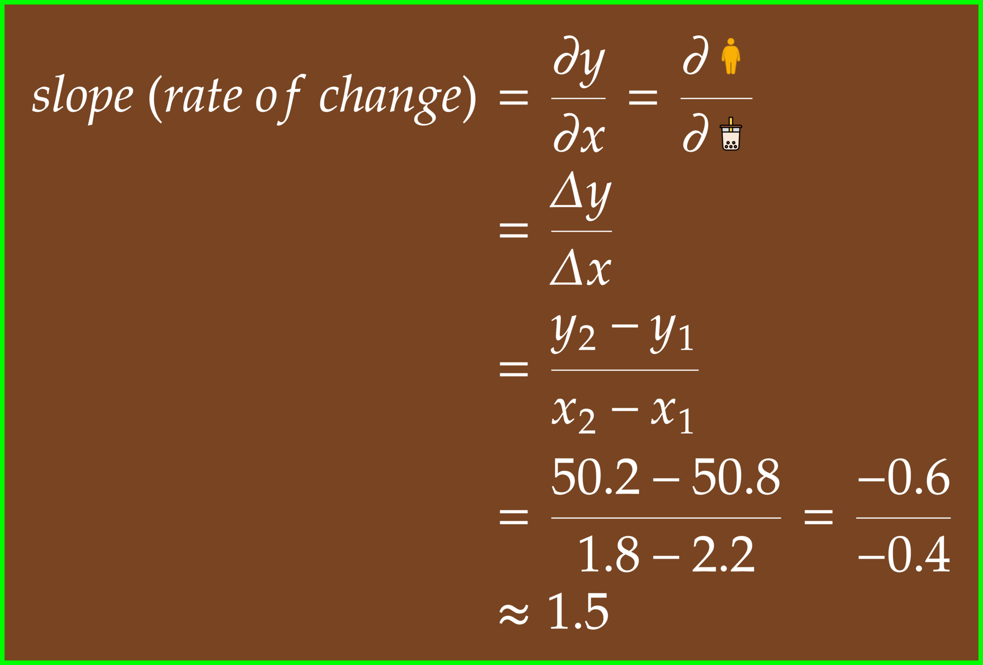
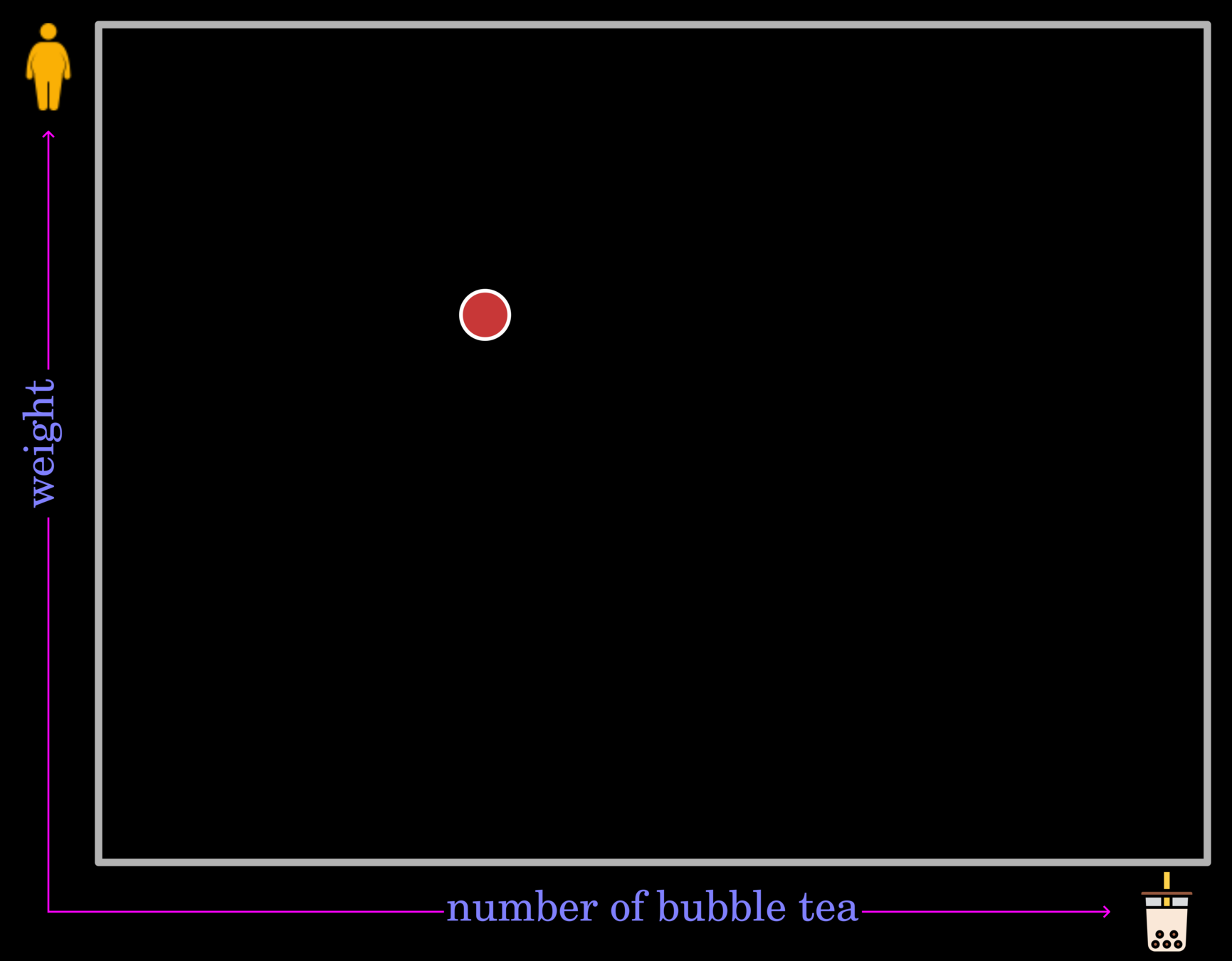
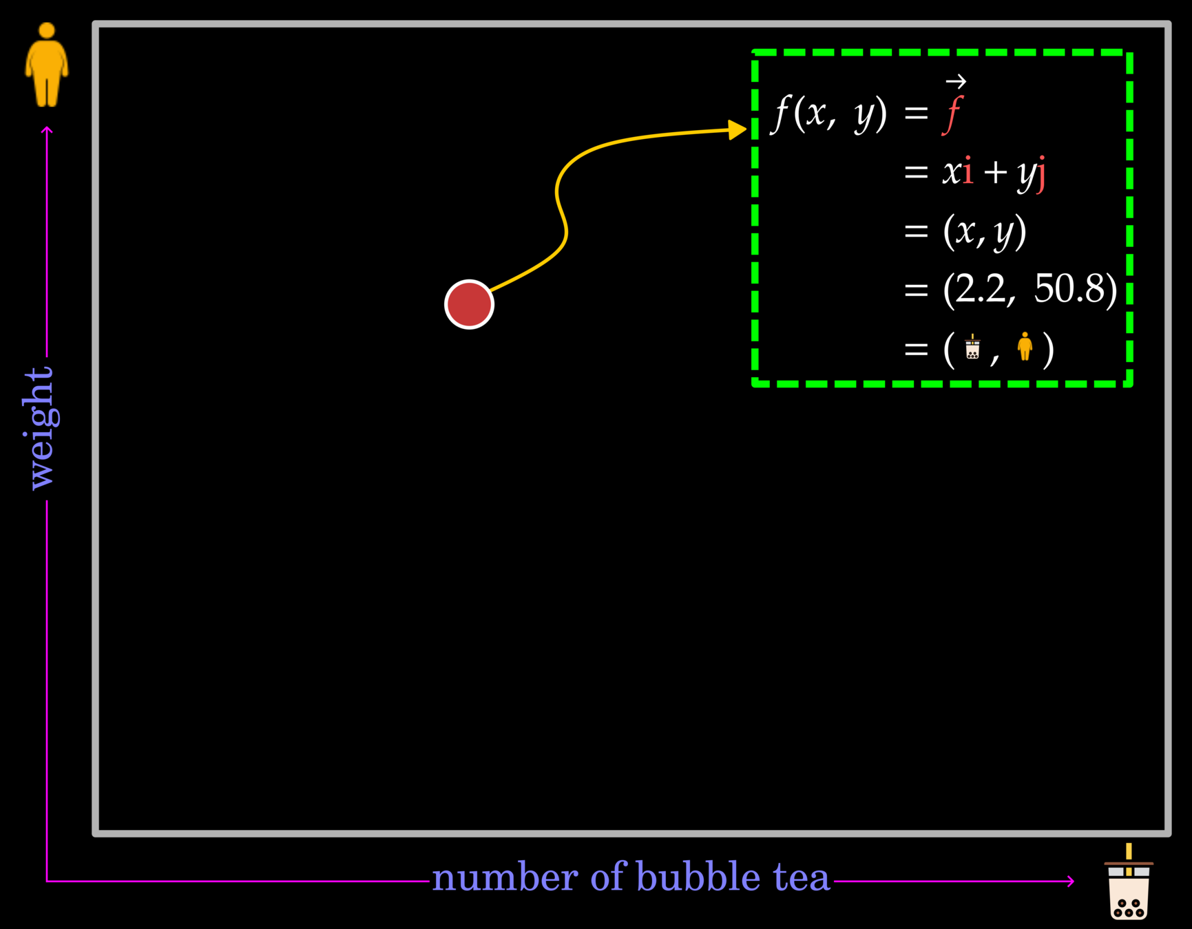
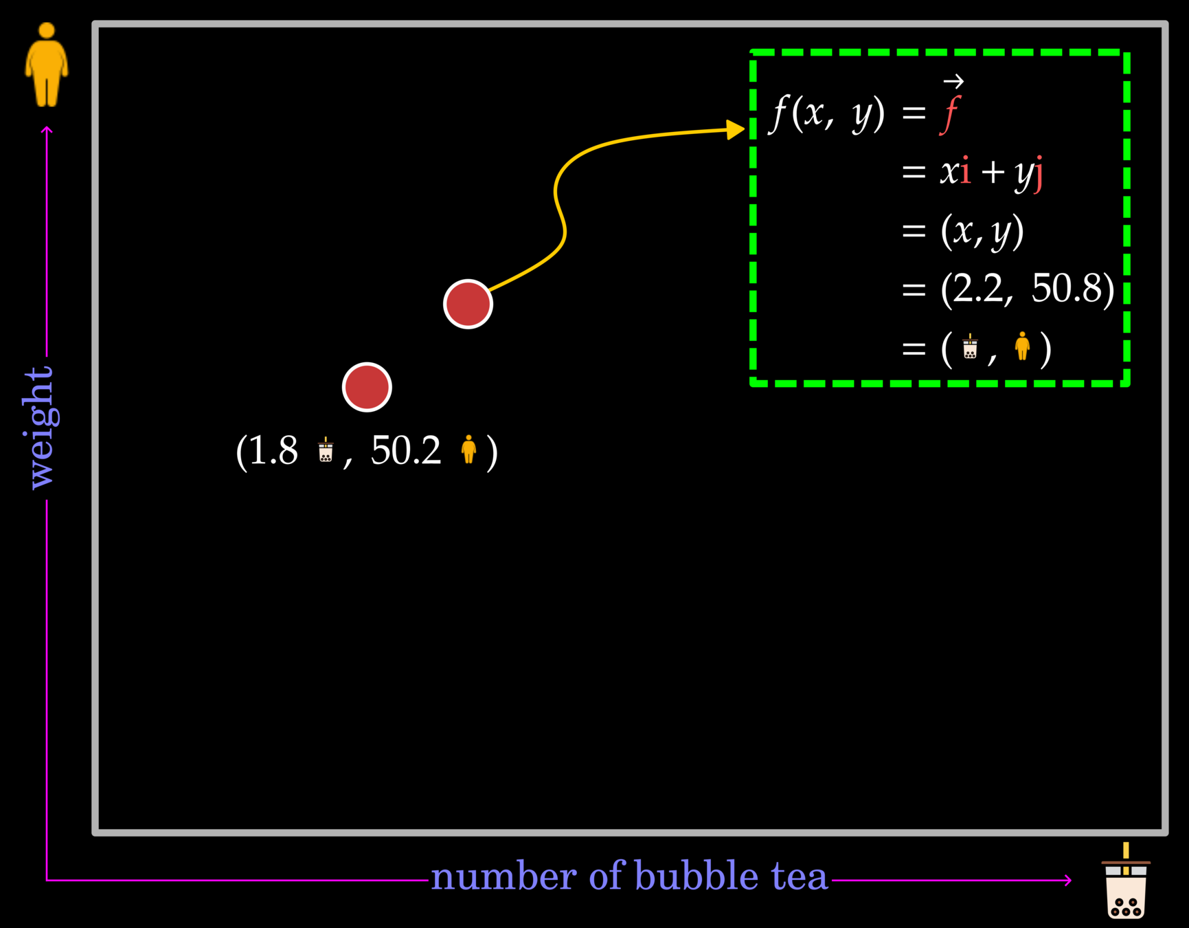
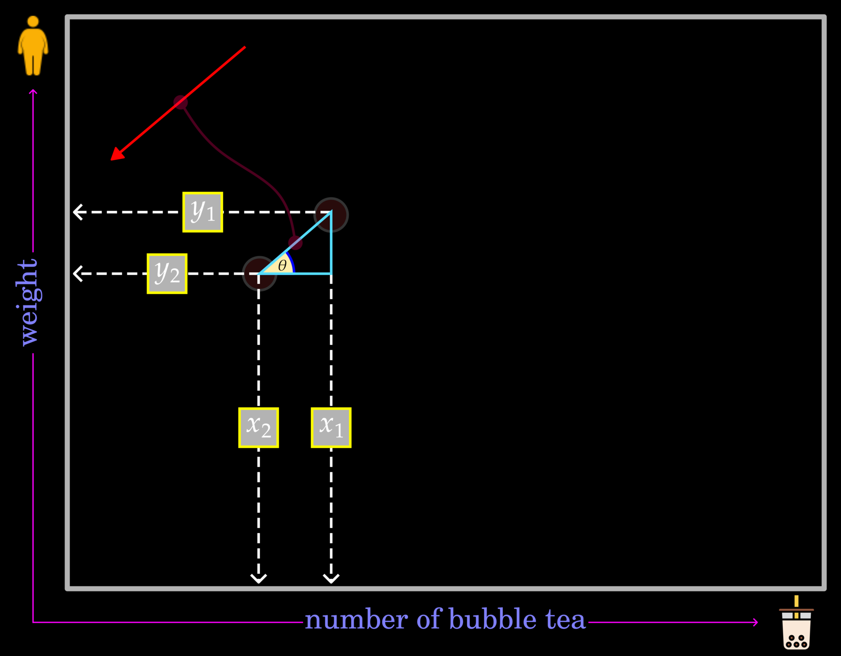
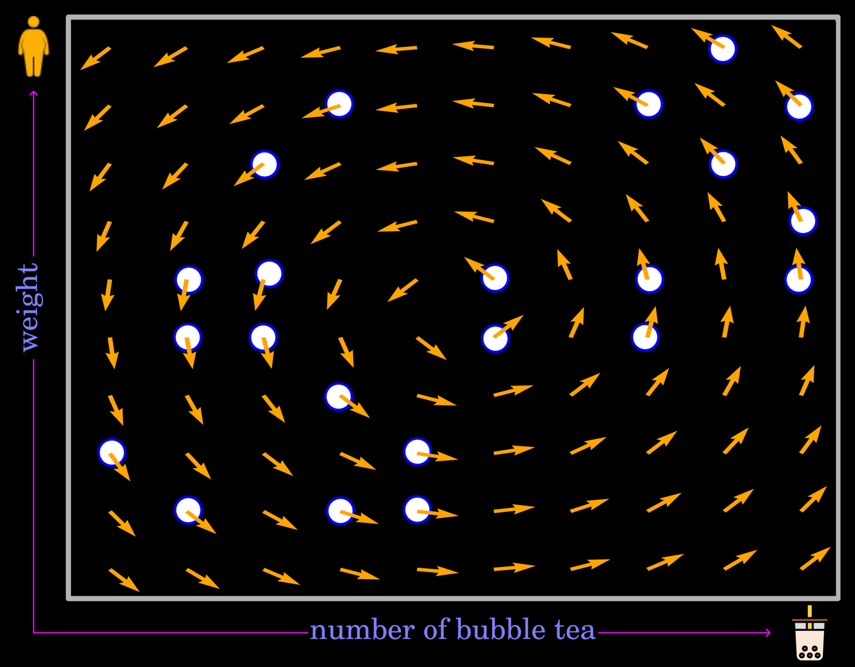
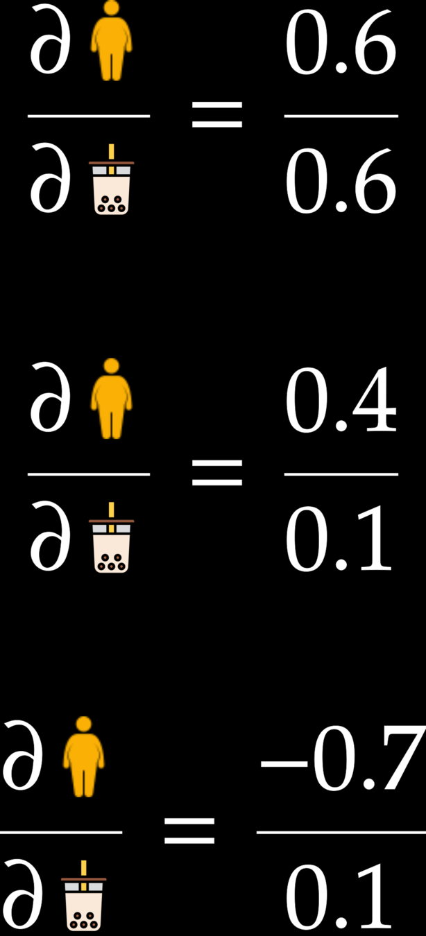
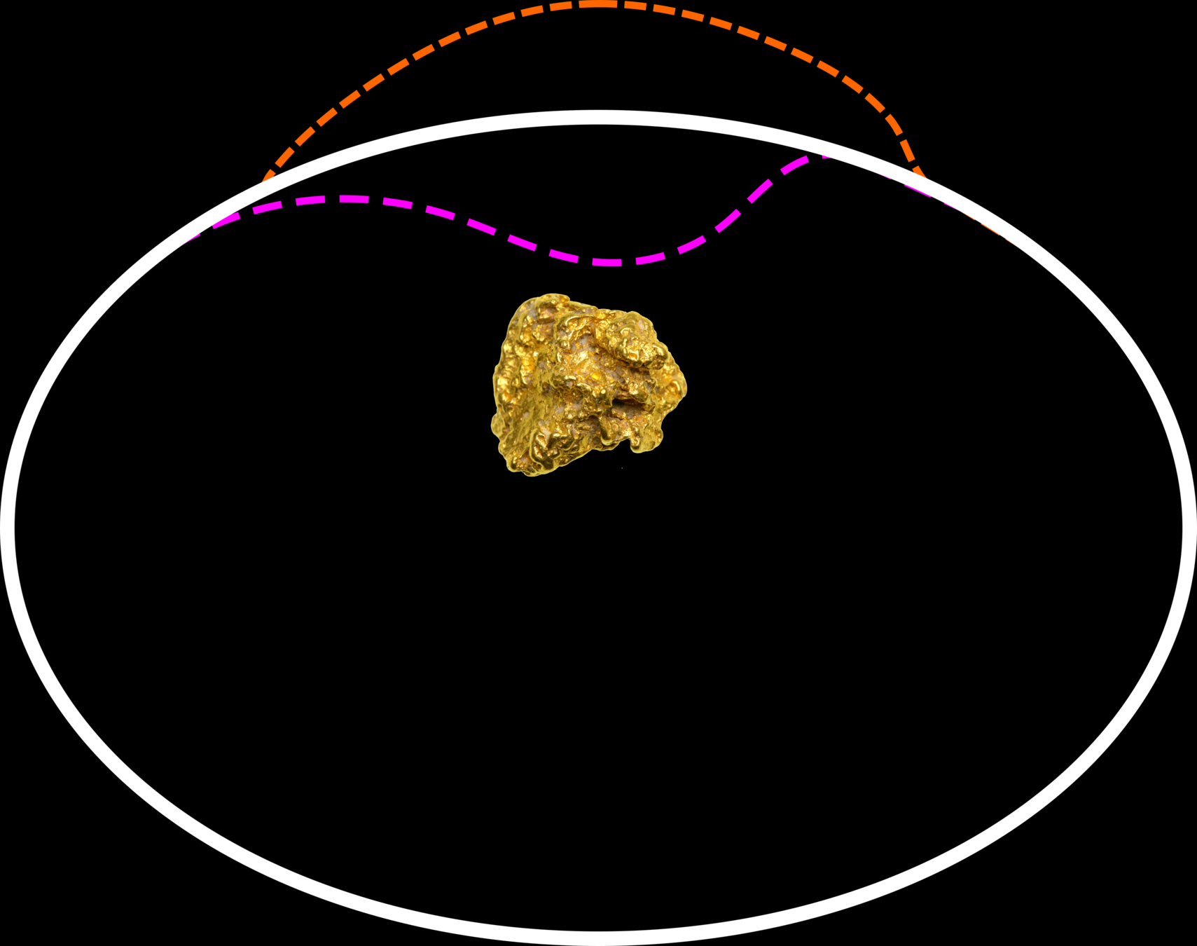
This example demonstrates the relationship between weight and the number of bubble tea in a space domain. The white dots indicate the observed data points.
Note that without probing a measuring device, we cannot confirm the existence of vector field. However, scientists can map a vector field based on observed stations, and this information will use for creating a function.
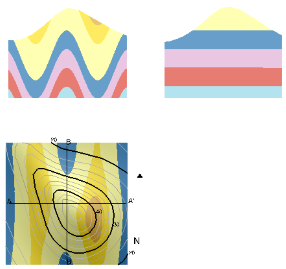
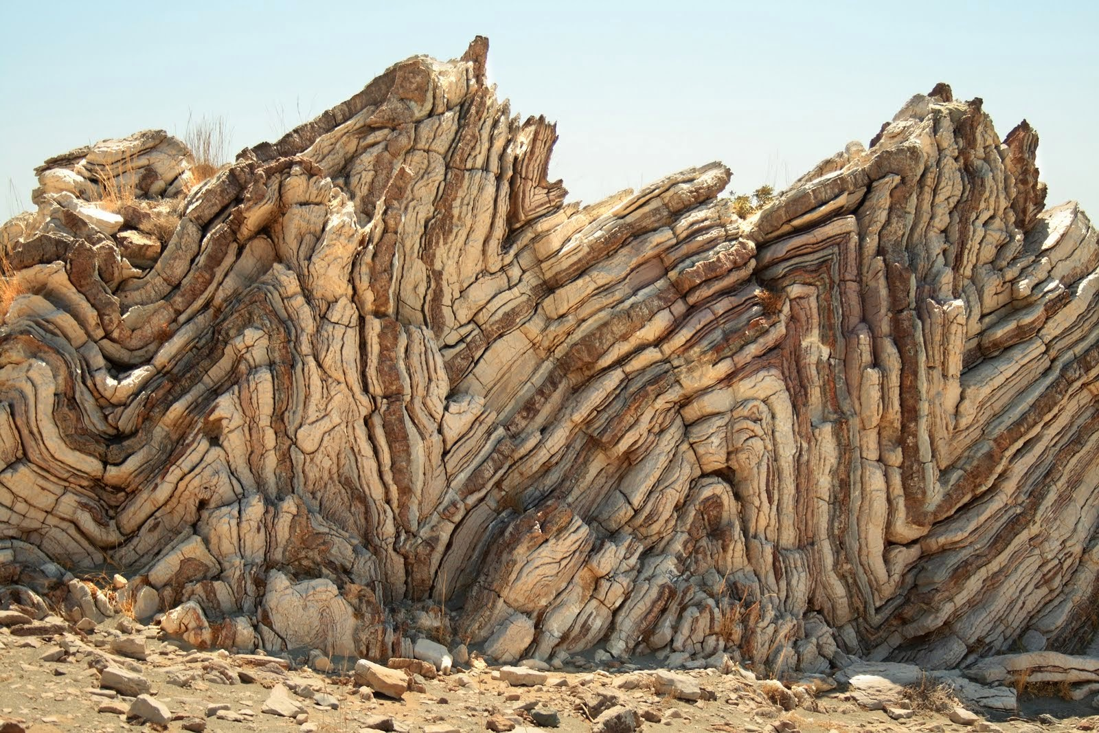
Geological Model
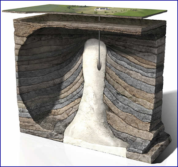
Potential Field Methods
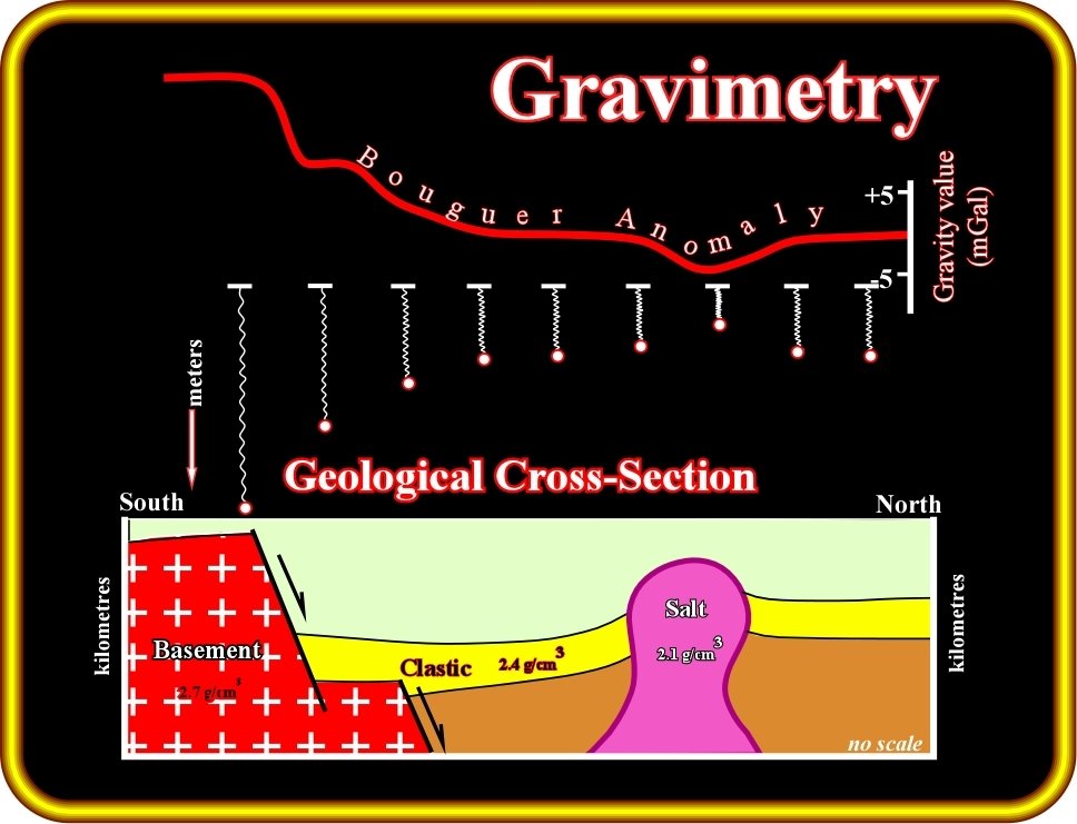
Gravimetry and Magnetics, i.e., the potential methods, are based on the potential theory. They have certain elements in common. Nevertheless their applications in oil exploration are quite different:
(i) Measured gravity effects are caused by sources that may vary in depth from the grassroots down.
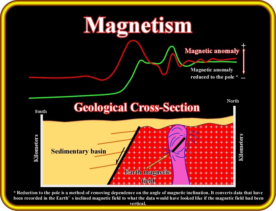
(ii) Sedimentary rocks, which are the ones in which generally hydrocarbon may occur, nearly always are less magnetic than the underlying basement (usually igneous or metamorphic rocks).
(iii) Magnetic effects are not too influenced by the sediments. One can say that its effects are almost the same as if the sediments were not present.
gravimetry
magnetism

Recap
| Material | Susceptibility x (SI) |
| Air | about 0 |
| Quartz | -0.01 |
| Rock Salt | -0.01 |
| Calcite | -0.001 - 0.01 |
| Sphalerite | 0.4 |
| Pyrite | 0.05 - 5 |
| Hematite | 0.5 - 35 |
| Illmenite | 300 - 3500 |
| Magnetite | 1200 - 19,200 |
| Limestones | 0 - 3 |
| Sandstones | 0 - 20 |
| Shales | 0.01 - 15 |
| Schist | 0.3 - 3 |
| Gneiss | 0.1 - 25 |
| Slate | 0 - 35 |
| Granite | 0 - 50 |
| Gabbro | 1 - 90 |
| Basalt | 0.2 - 175 |
| Peridotite | 90 - 200 |
10^{-3}
Use the table on the left to select one rock with the possibility of having the highest magnetic susceptibility.
1. Submit the BT median (magnitude of magnetic field) via slack. We use the median rather than the mean to avoid anomaly and spiking data.
Simple Harmonic
1 hertz = 1 Hz = 1 oscillation per second = 1 s
-1

T = \frac 1 f
2\lambda = T
amplitude

phase\ angle\ \theta\ =\ 0
Use the Harmonic equation to reproduce the cosine function shown in the figure above. Try to modify the parameters such as amplitude, frequency, and phase. You might superimpose your results to analyze what differences are.
Applied Harmonic to Measuring Singal in Geophysics

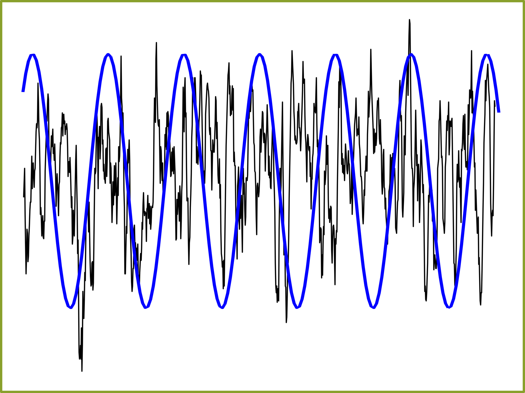
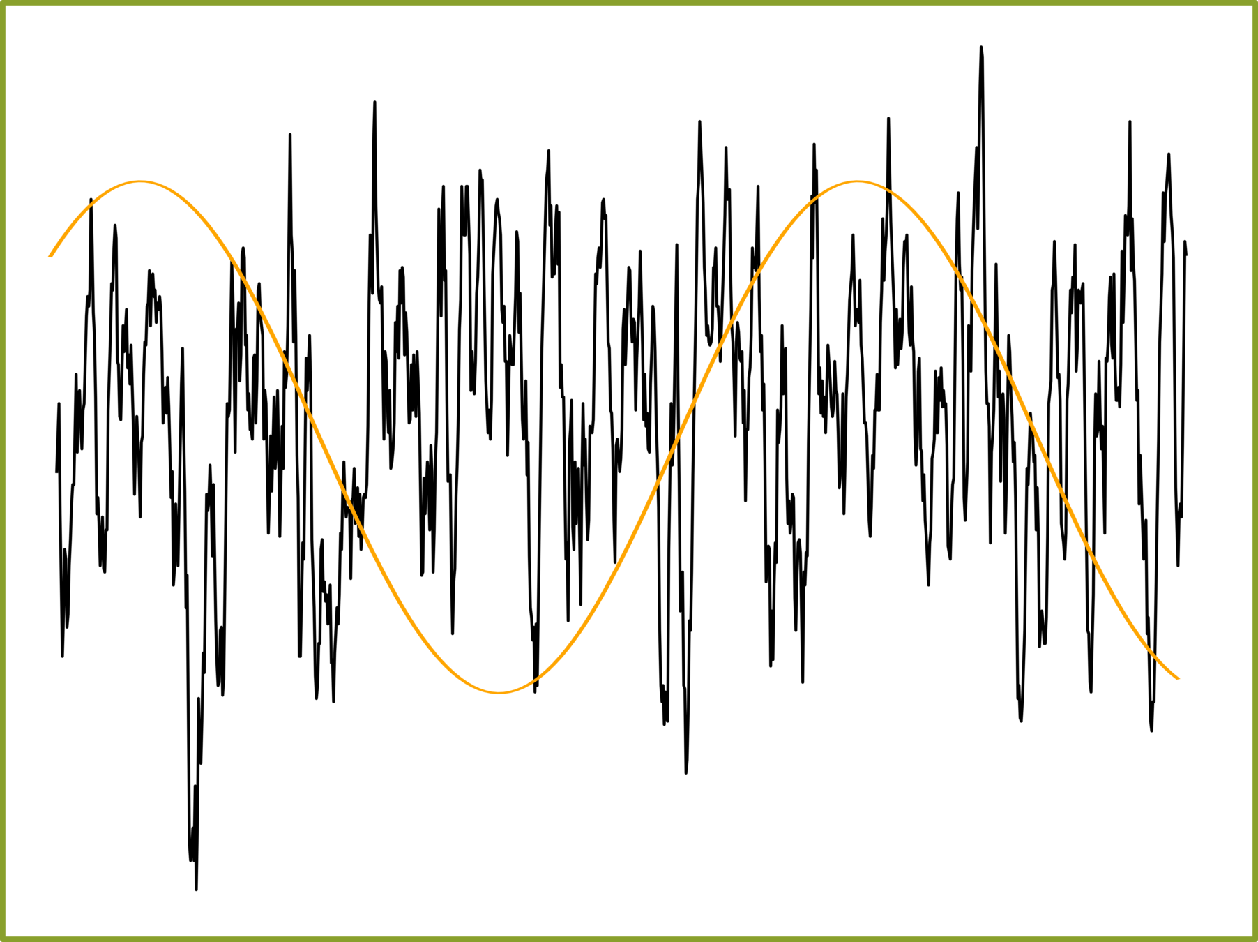


Image Resolution
Mean, Median, Mode, and Percentile

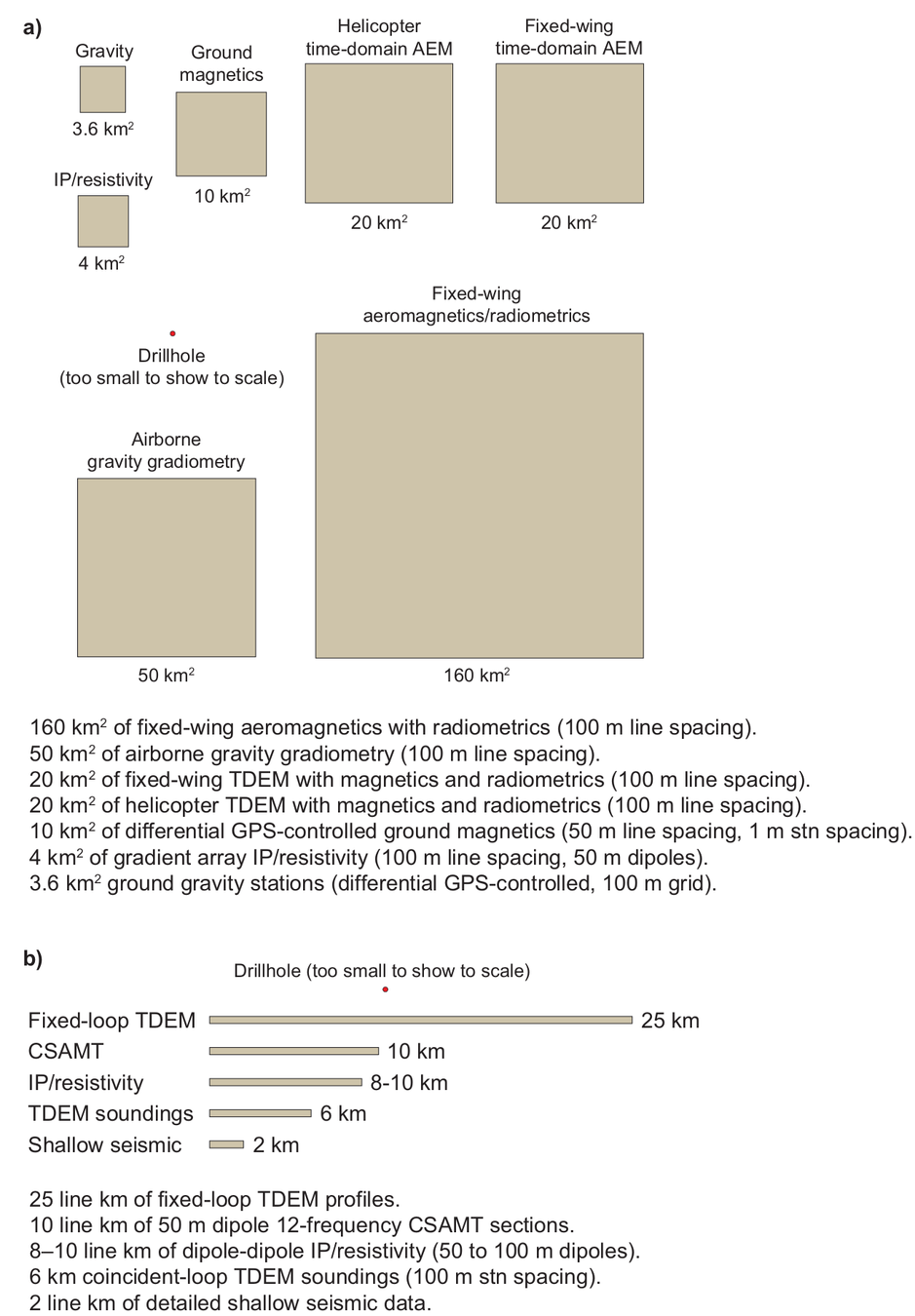
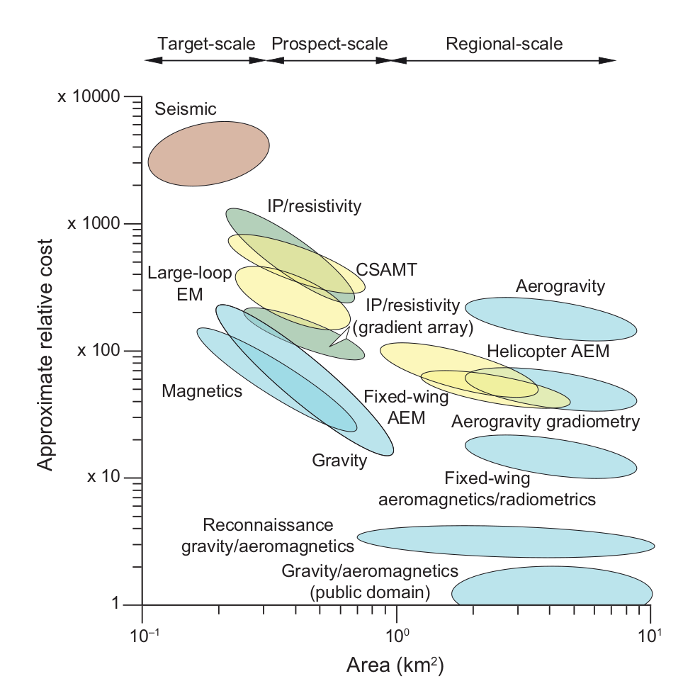
Geophysical Servey and Resolution
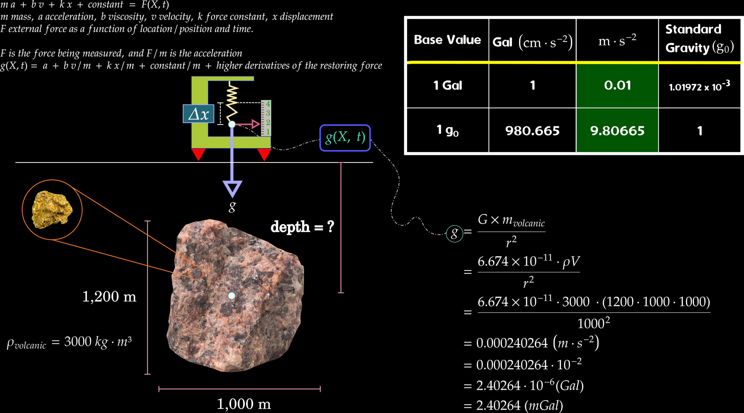
Newton's Law of Universal Gravity
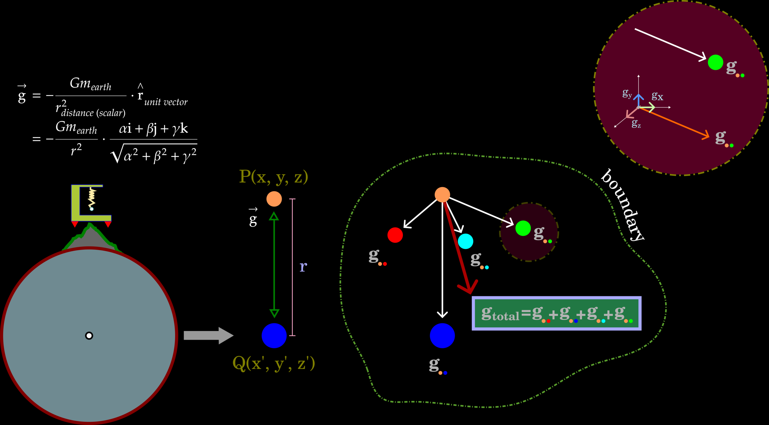
Newton's law of universal gravitation describes the relationship between mass attractions and forces shown as (1). We can derive the Earth’s gravitational field (3) based on the relationship between(1) and Newton's second law (2).
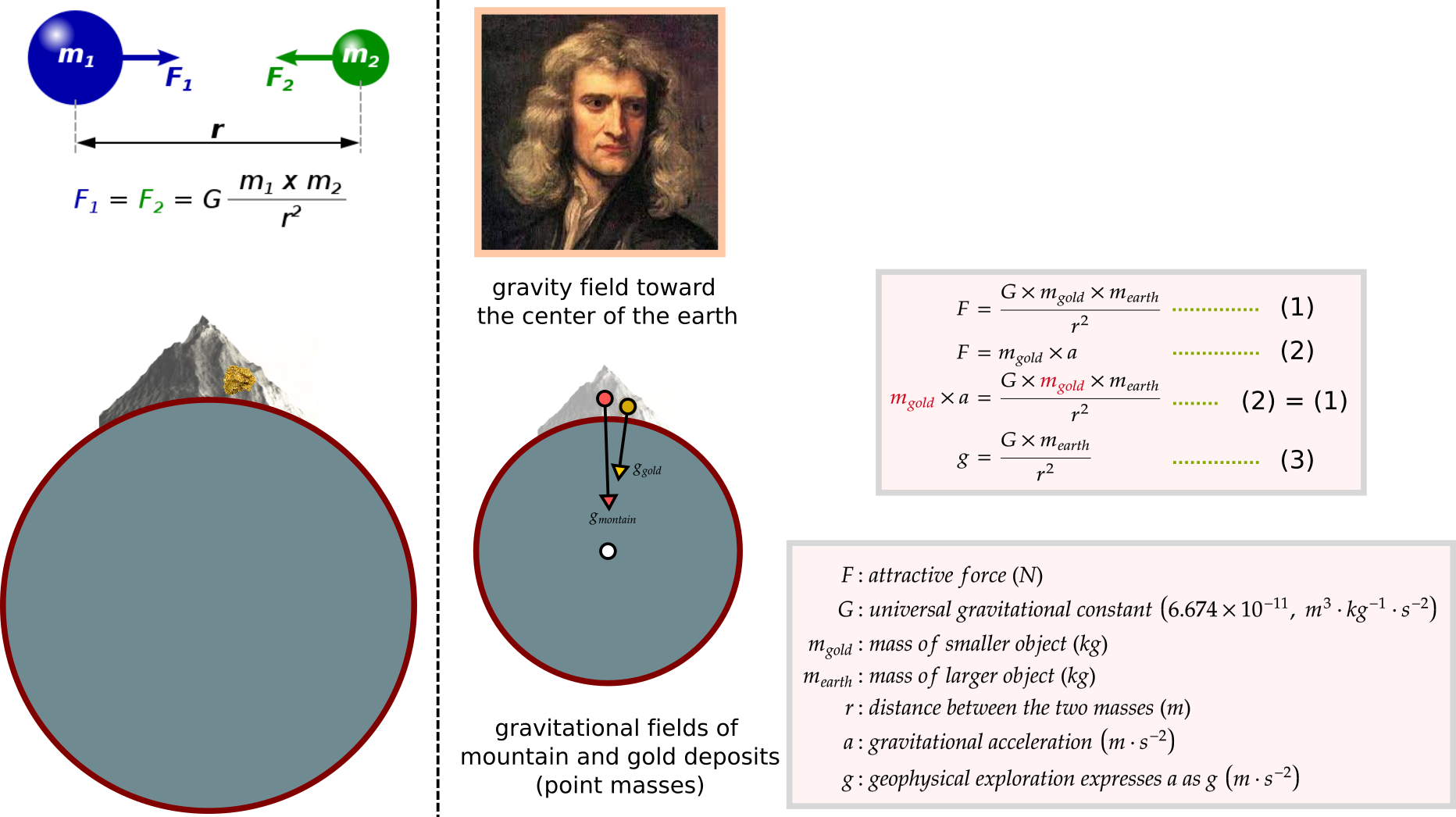
Earth's gravity decreases when increasing the distance from the center of the earth. Based on the gravity equation, please demonstrate how the gravity strength decreases with increasing distance from the center of the earth.

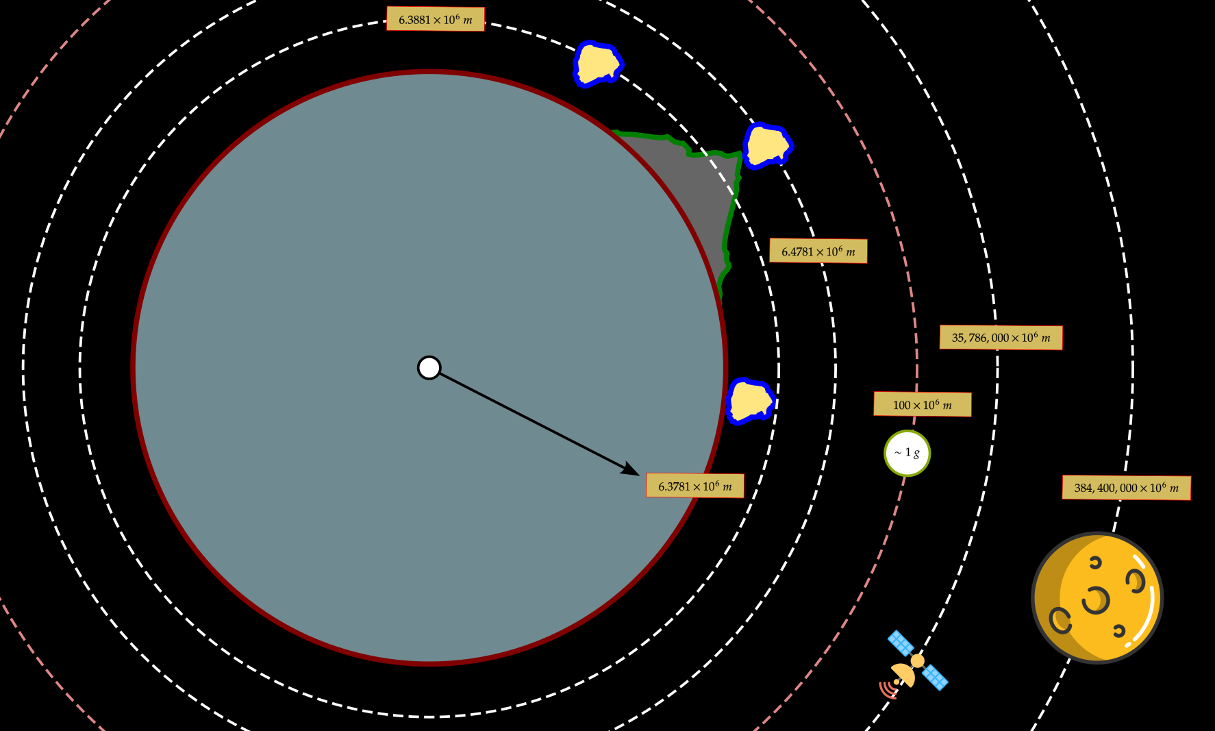

Task 1: Using the earth's gravitational equation to reproduce the figure above. Students may study the code snippet below for the guild line.
1. When will gravity attraction has acceleration less than 1 ?
2. Near the earth's surface, how much variation of the gravity accerlation.

Gravity Units
The Shape of the Earth: Ellipsoid
Assumption
1. Shape of the earth is a spheroid.
2. Earth's material is homogeneous.
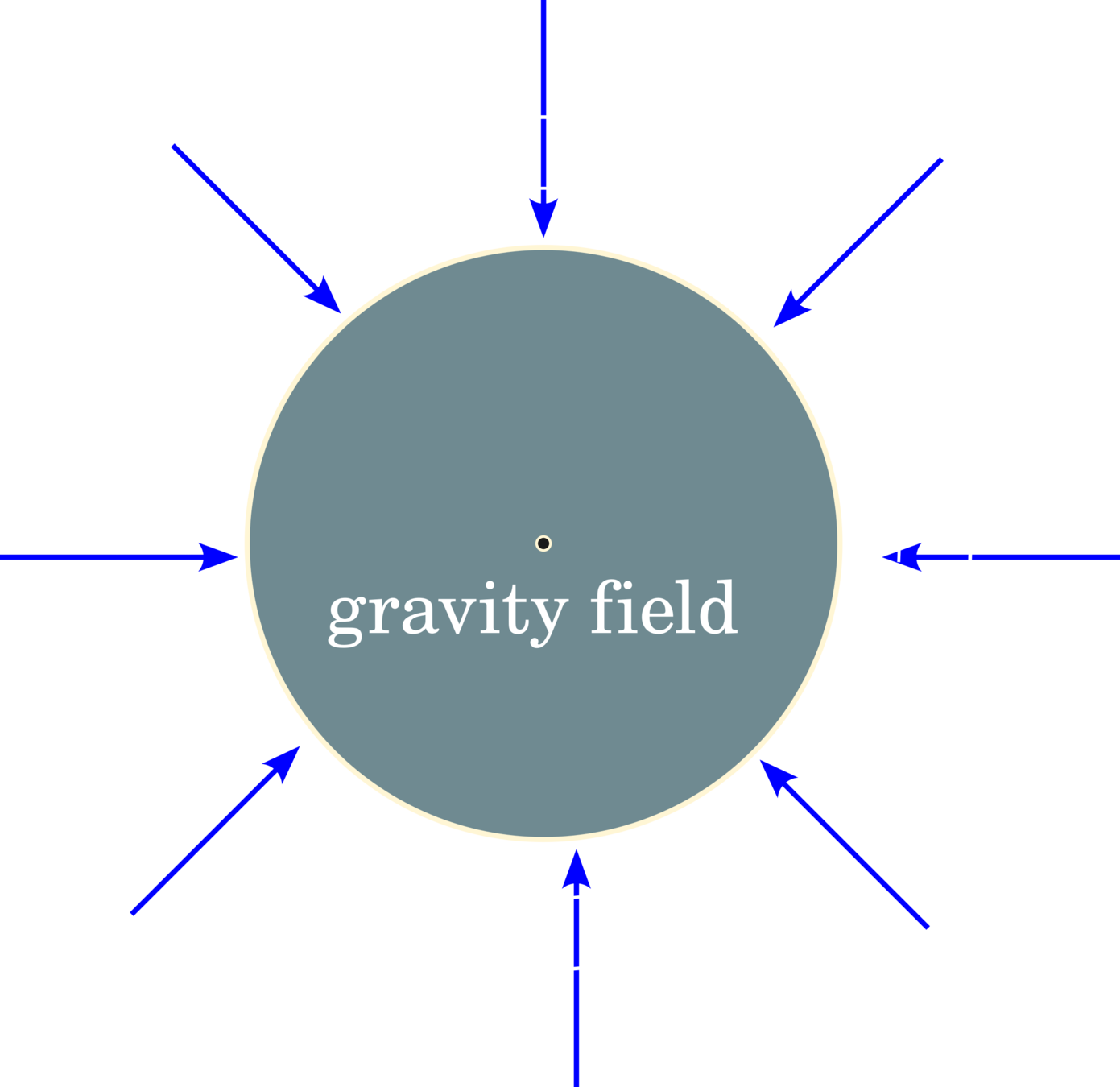
This assumption leads to maximum gravity intensity near the earth's surface and will reduce the intensity when the distance increases from the earth's center.
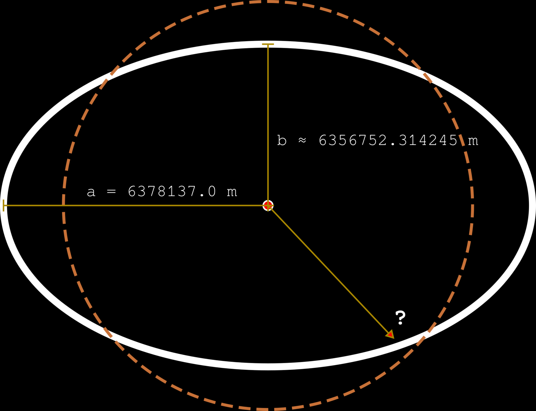
We know that shape of the earth is likely oblate spheroid (ellipsoid). The ellipsoid approximation can refer to the reference ellipsoid, World Geodetic System (WGS), using model WGS 84.
Simplified World Geodetic System (WGS)

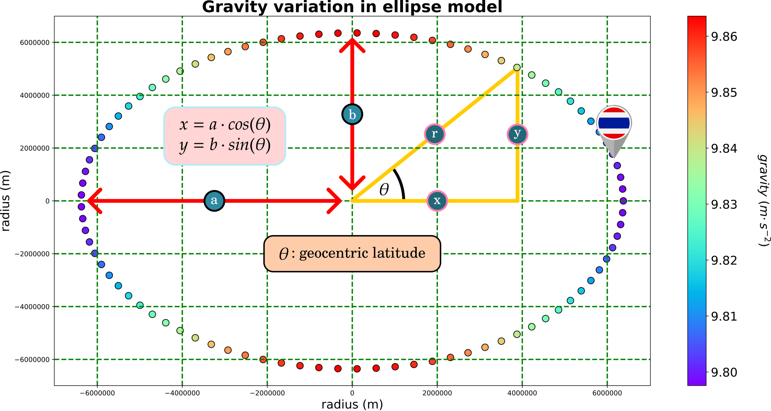
Task: reproduce this figure and compute gravity in Thailand
(latitude 15 degrees) using an ellipse parametric equation.
Gravity as a Vector: Point Mass
Gravity is a vector field, so a mass unit in a gravimeter will experience multiple gravitational attractions from multiple positions. The reading values represent the magnitudes of the total gravity field. Typically, this refers to g(z) pointing toward the earth's center.
The earth materials are not unit points, and they are likely heterogeneous. Hence, this concept needs more assumptions to tackle the subsurface imaging problems.
Applied Point Mass Concept into Geophysics Problems
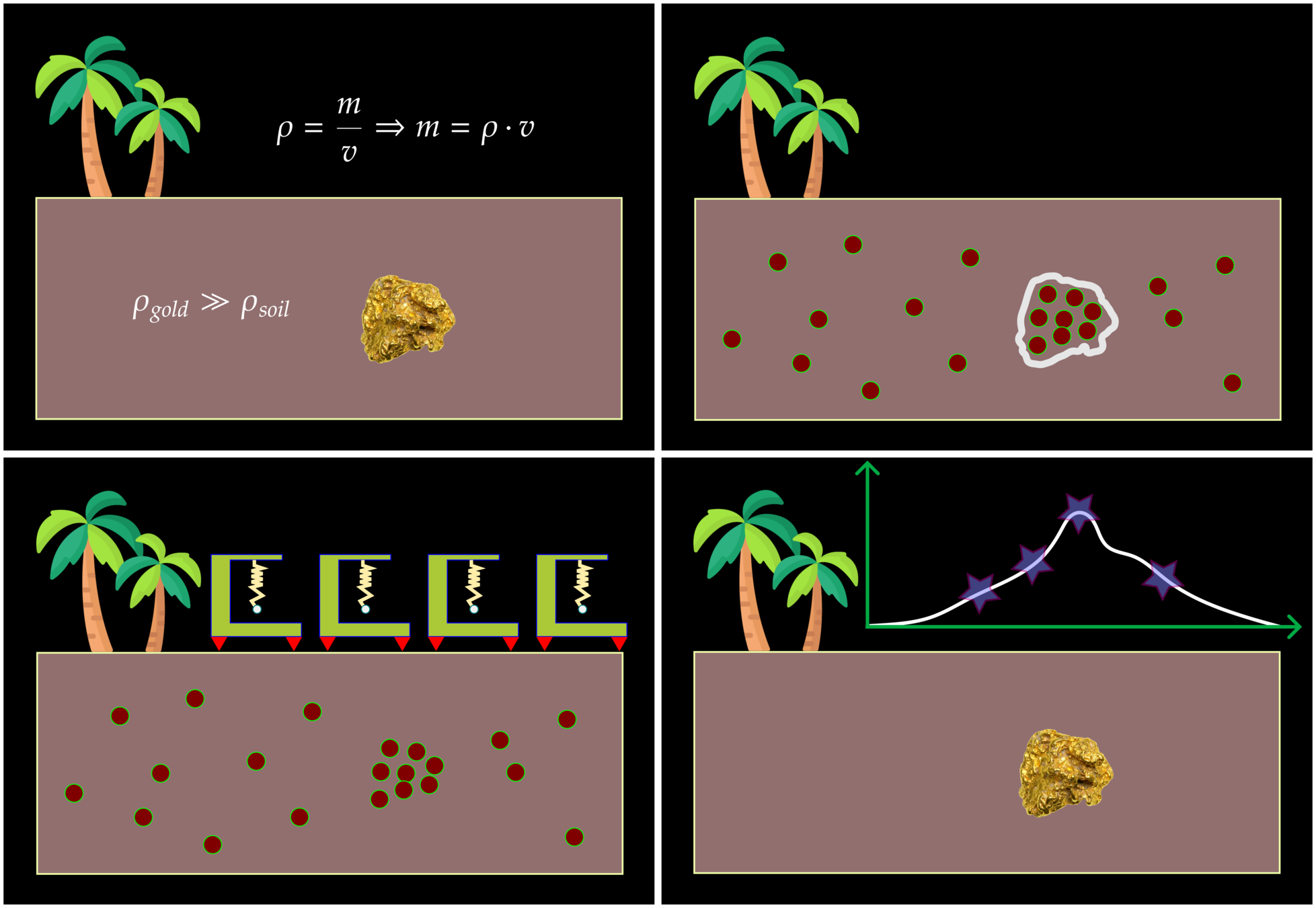
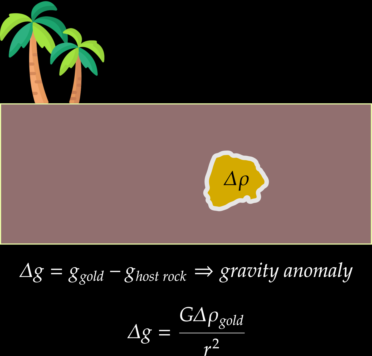
This assumption leads to density contrasts (excess mass) in which the ore deposit has more density than the host rock. The gravimetry will read gravitational accerlation adjacent to the ore deposit as an anomaly.
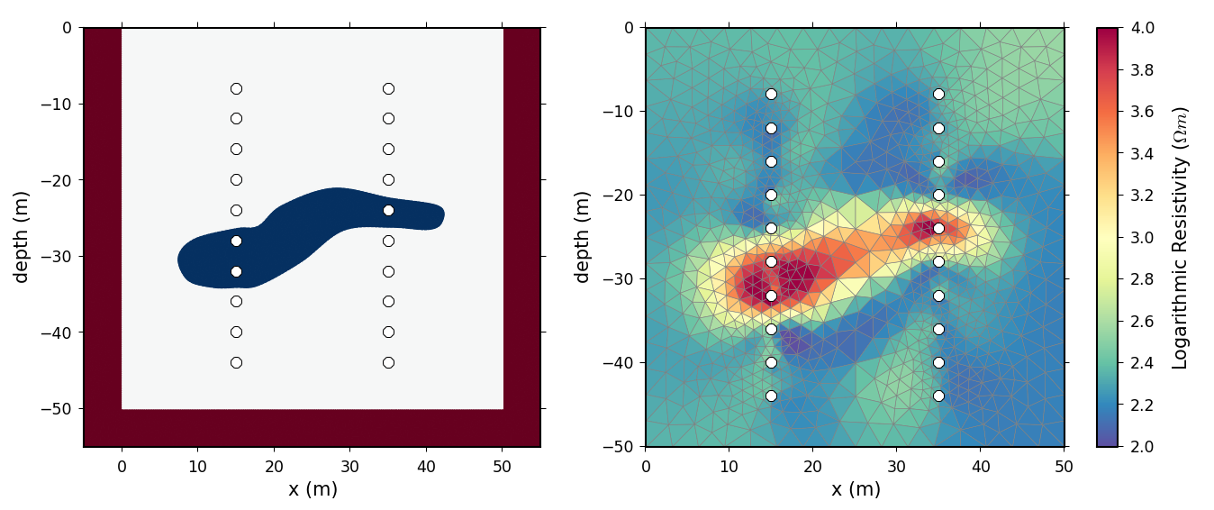
Forward Modeling Gravity: Sphere
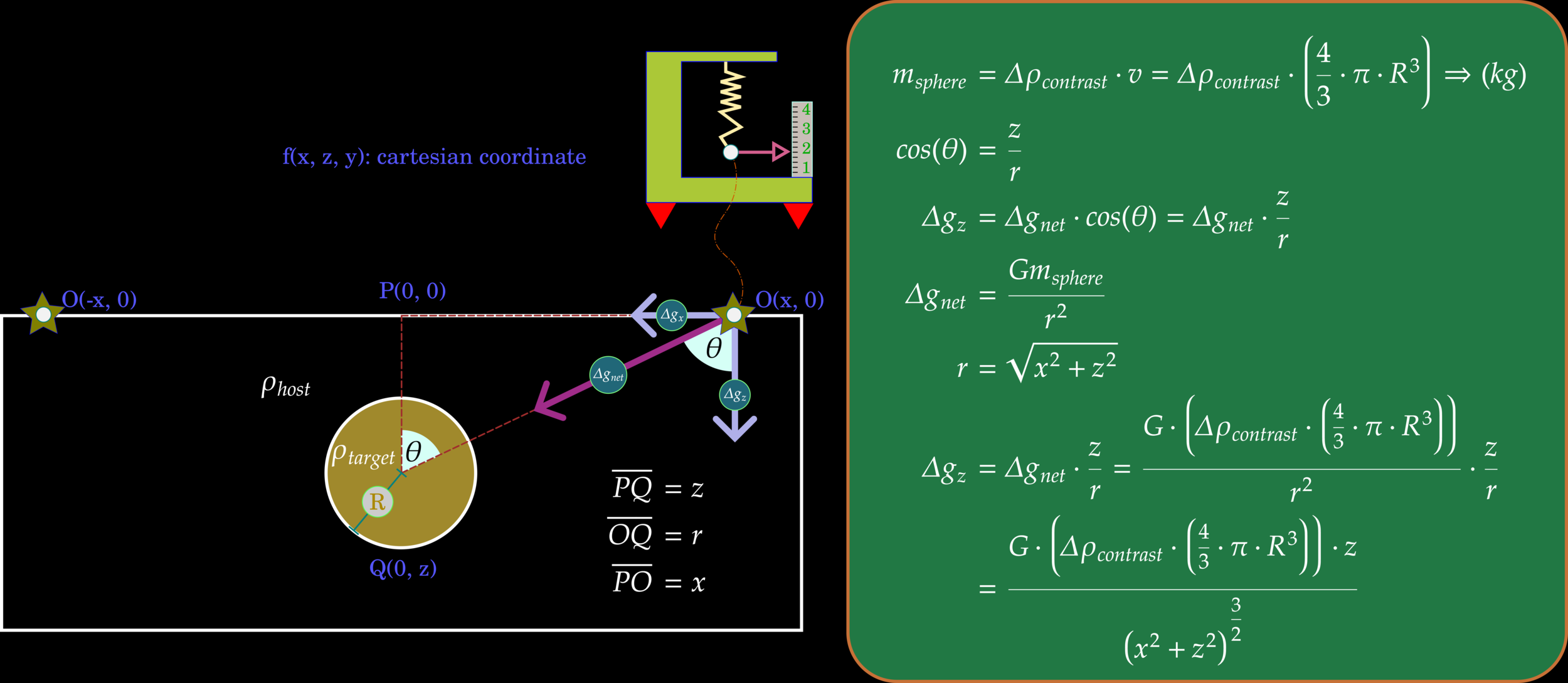
Suppose our observation target in the subsurface is a buried sphere, and we focus the gravitational attraction only on axis-z. Thus, this task can approximate into a 2D problem, in which derived equations are shown on the RHS.
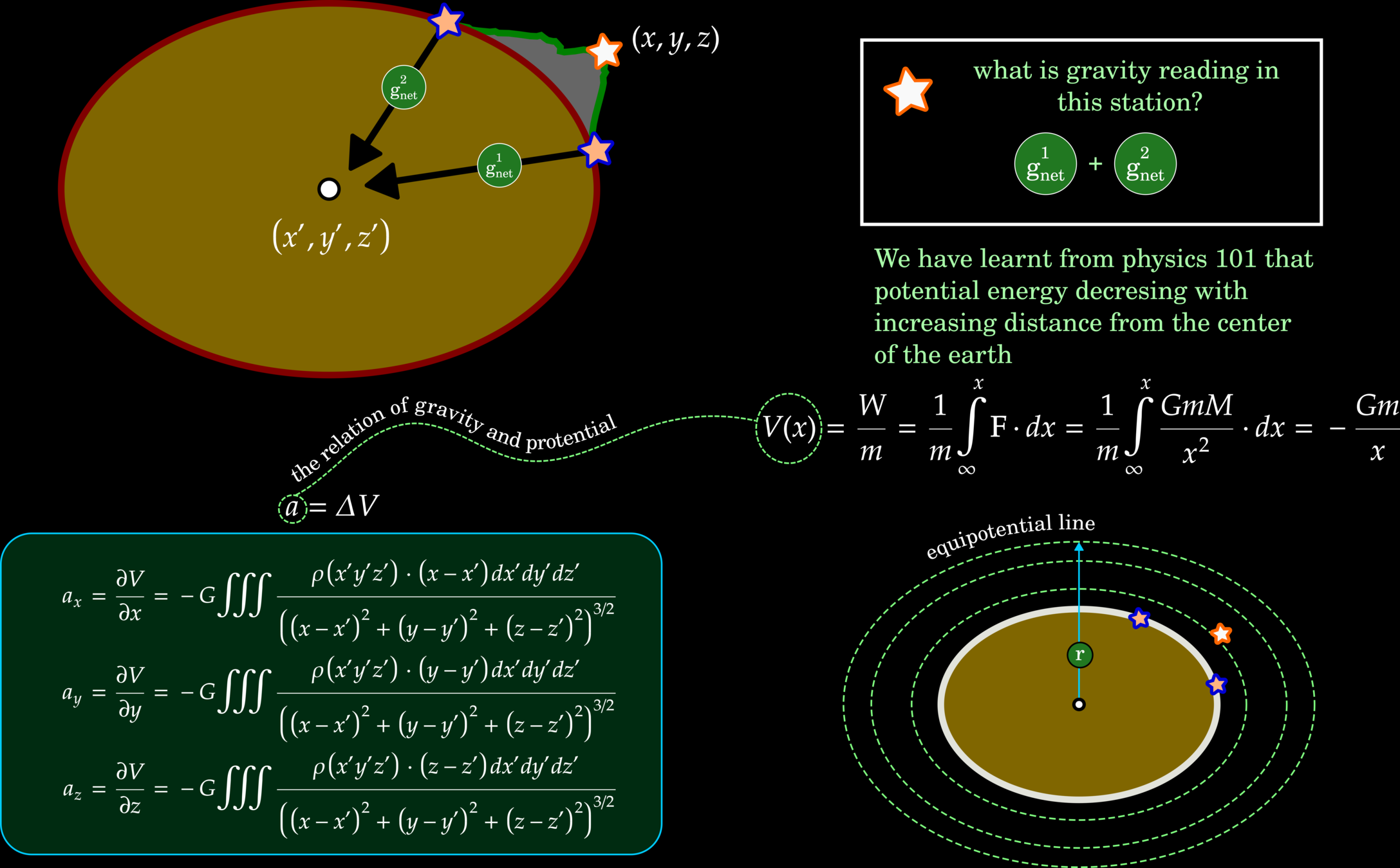
Forward Modeling Gravity: Irregular Shapes
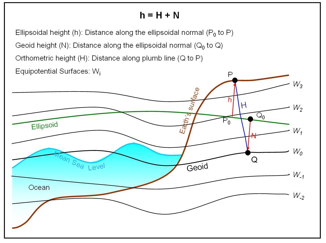
Gravitational Potential
Mean Sea Level
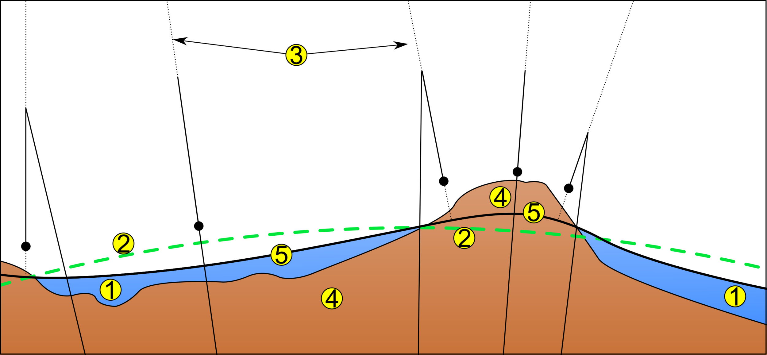
1. Ocean, 2. Reference ellipsoid, 3. Local plume line, 4. Continent, 5. Geoid
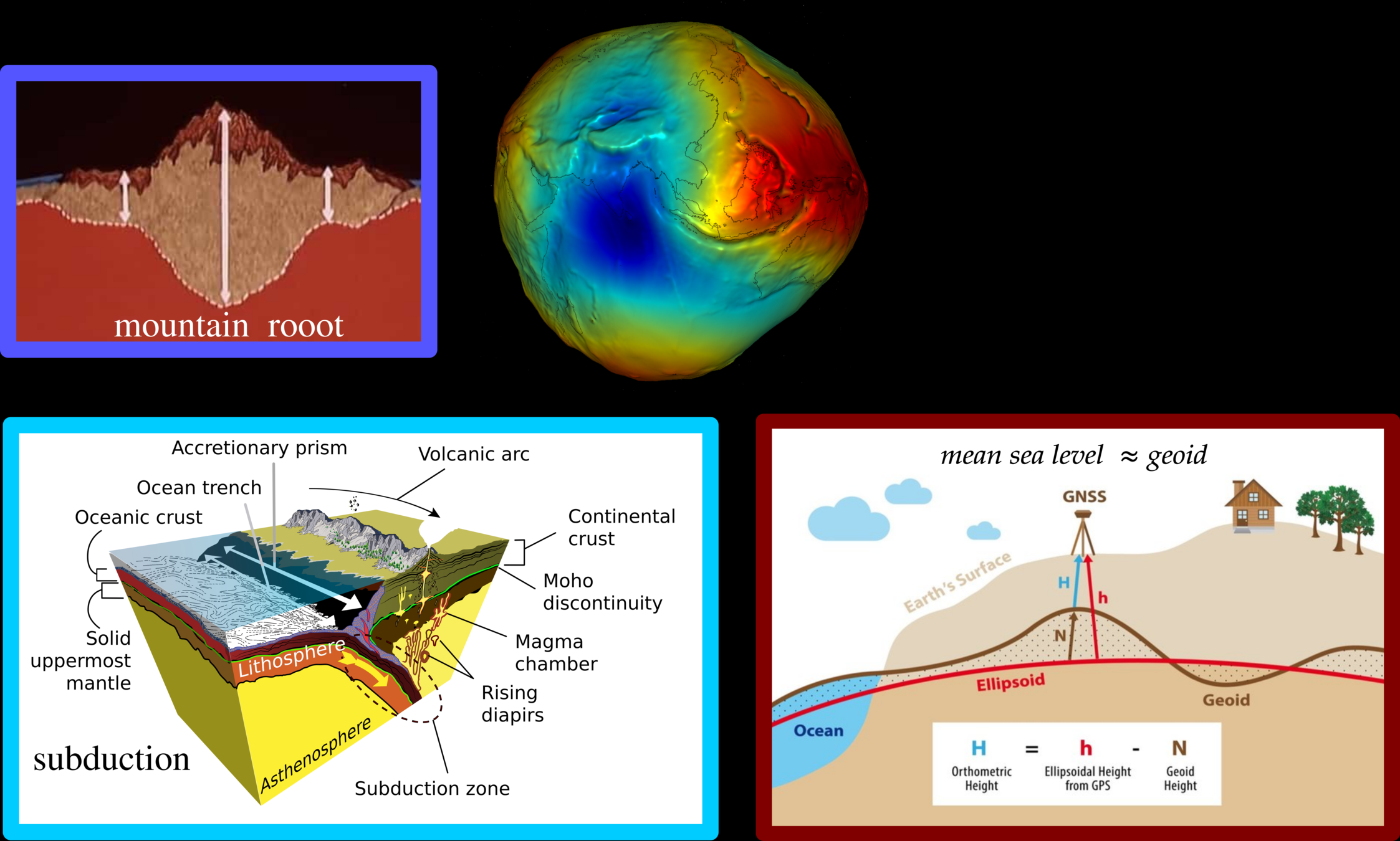
Geoid: Earth's Subsurface is Heterogeneous
The geoid is the shape that the ocean surface would take under the influence of the gravity of Earth, including gravitational attraction and Earth's rotation, if other influences such as winds and tides were absent. This surface is extended through the continents (such as with very narrow hypothetical canals). According to Gauss, who first described it, it is the "mathematical figure of the Earth", a smooth but irregular surface whose shape results from the uneven distribution of mass within and on the surface of Earth.[1] It can be known only through extensive gravitational measurements and calculations
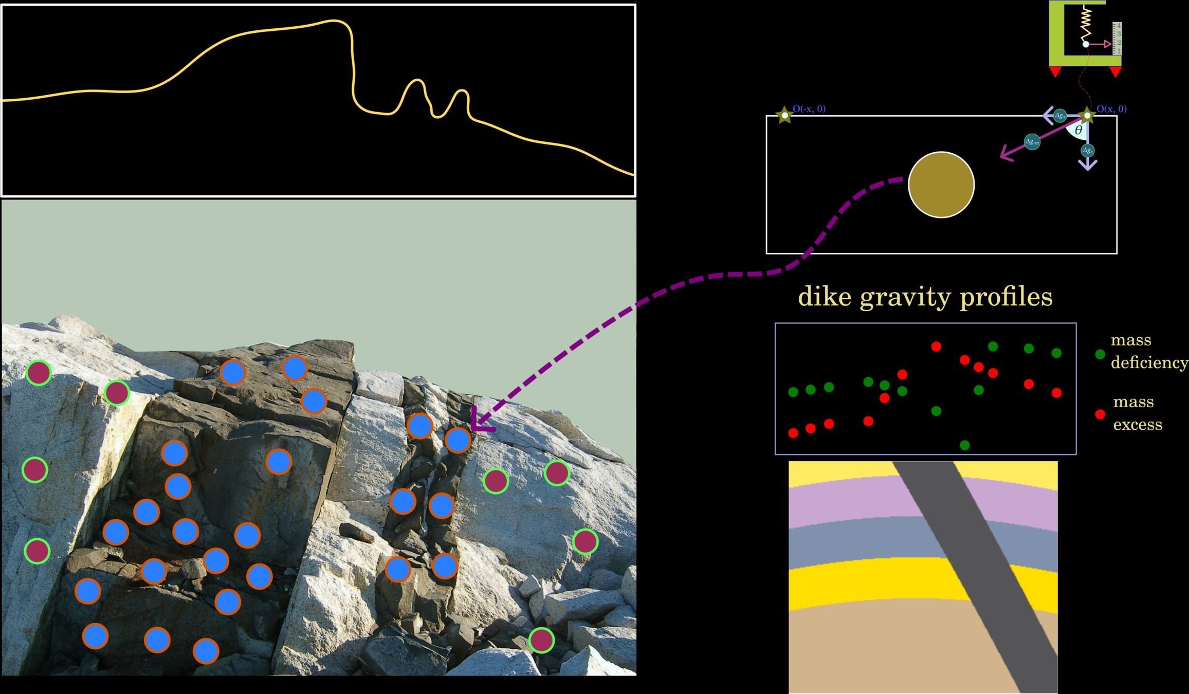
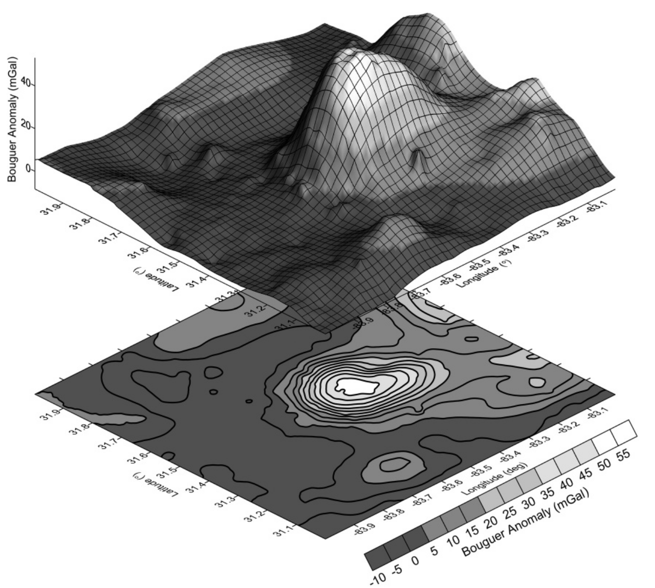
Gravity Anomaly
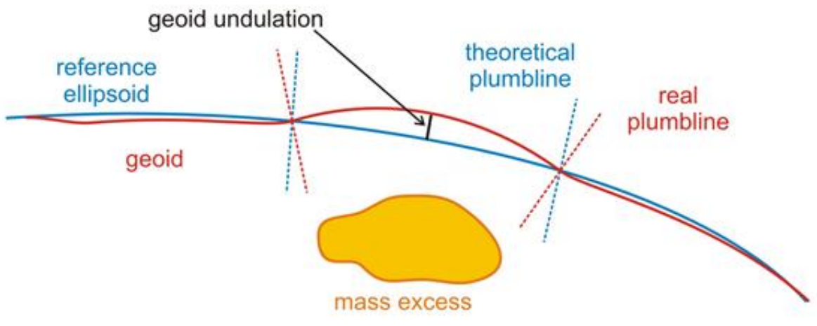
The gravity anomaly at a location on the Earth's surface is the difference between the observed value of gravity and the value predicted by a theoretical model. If the Earth were an ideal oblate spheroid of uniform density, then the gravity measured at every point on its surface would be given precisely by a simple algebraic expression. However, the Earth has a rugged surface and non-uniform composition, which distorts its gravitational field. The theoretical value of gravity can be corrected for altitude and the effects of nearby terrain, but it usually still differs slightly from the measured value. This gravity anomaly can reveal the presence of subsurface structures of unusual density. For example, a mass of dense ore below the surface will give a positive anomaly due to the increased gravitational attraction of the ore.

Different theoretical models will predict different values of gravity, and so a gravity anomaly is always specified with reference to a particular model. The Bouguer, free-air, and isostatic gravity anomalies are each based on different theoretical corrections to the value of gravity.

A gravity survey is conducted by measuring the gravity anomaly at many locations in a region of interest, using a portable instrument called a gravimeter. Careful analysis of the gravity data allows geologists to make inferences about the subsurface geology.
mass excess and deficiency
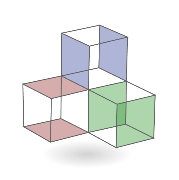
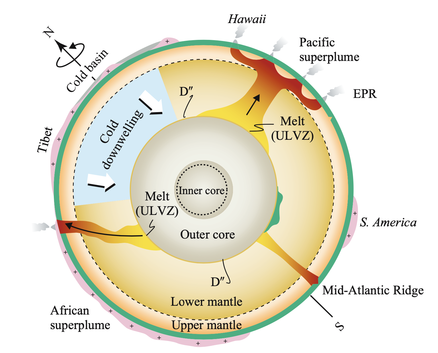
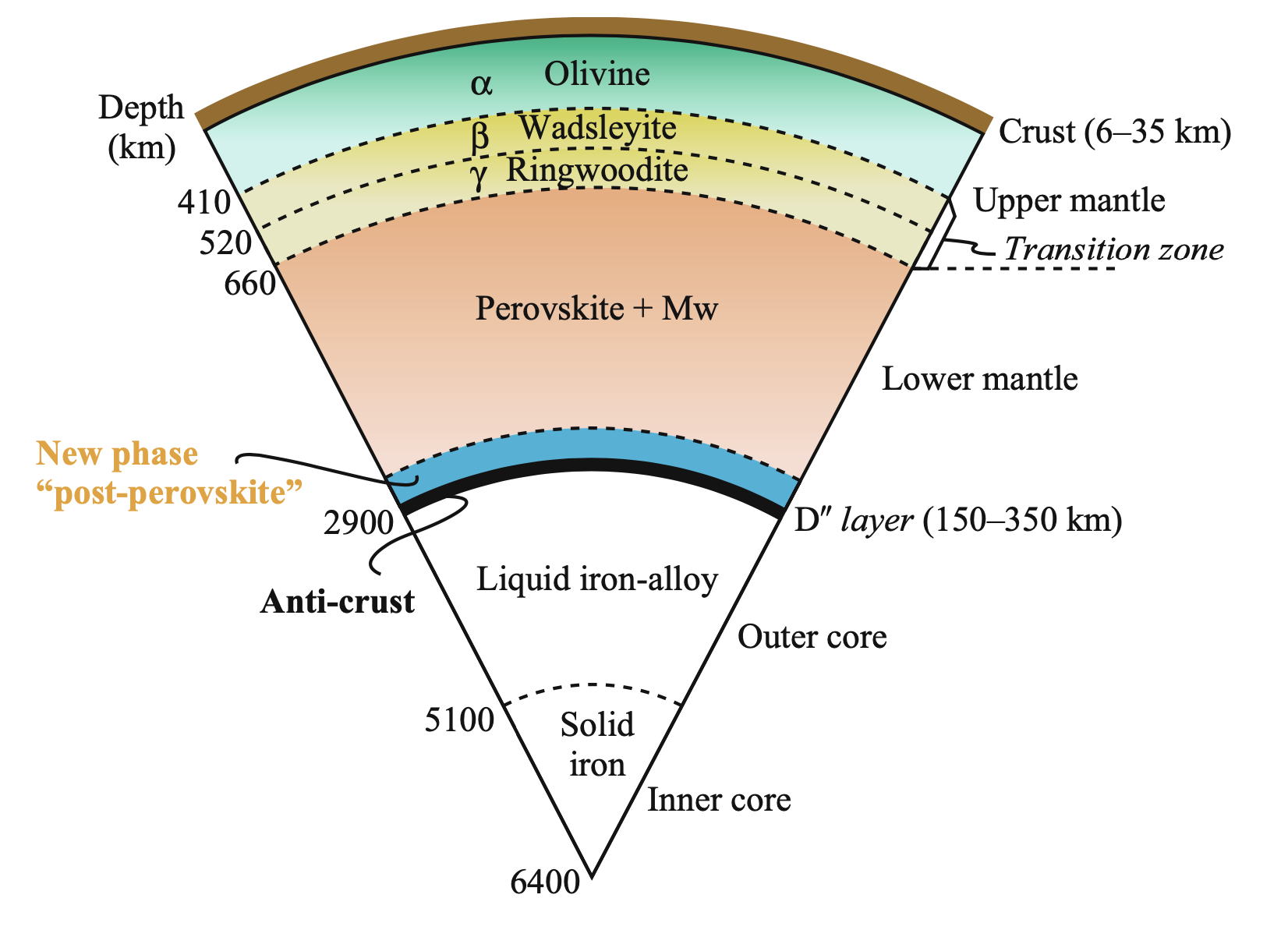
The Onion Earth
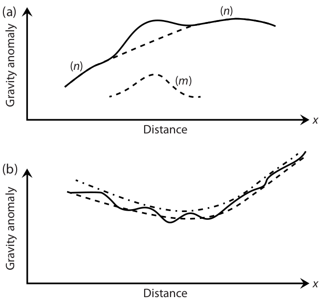
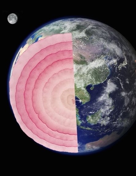
simple
complex
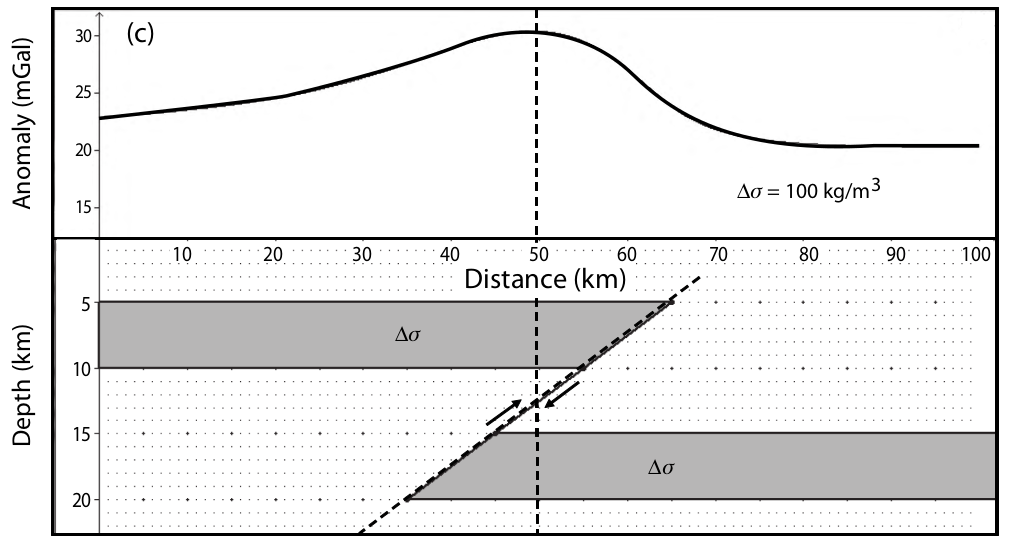
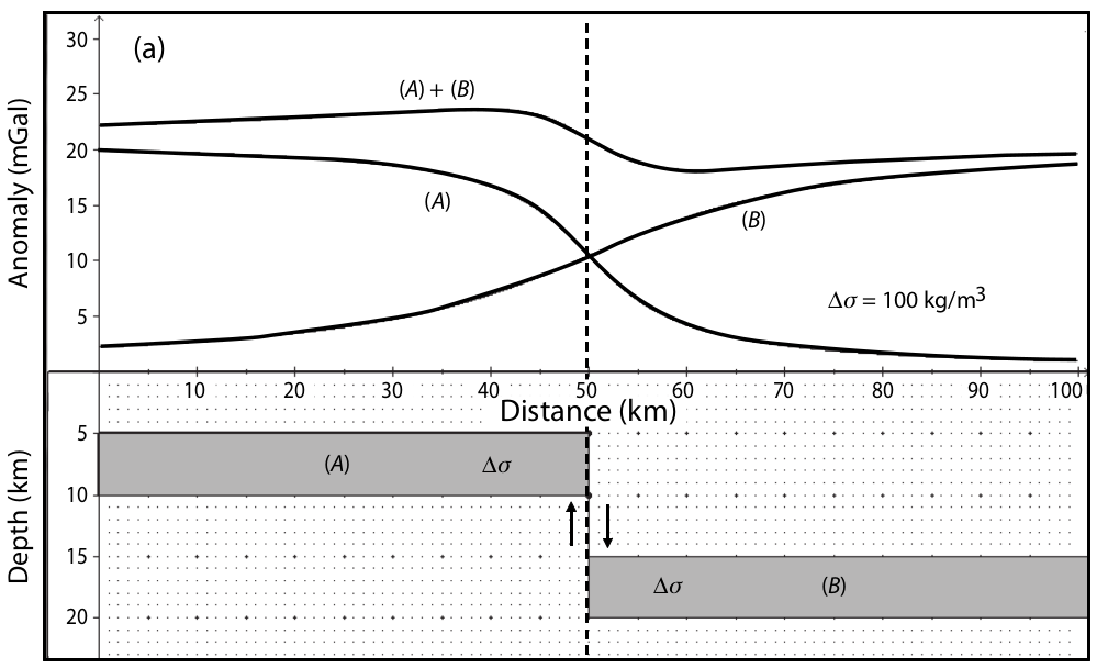
Gravity exploration in geophysics is a superposition of the multilayer of the earth's structure. The gravity reading is a summation of gravity, which requires collection methods to separate between target and background. Modeling and inversion are typical methods that geophysicists use to decompose the earth's statra.
Gravity Interpretation
Density
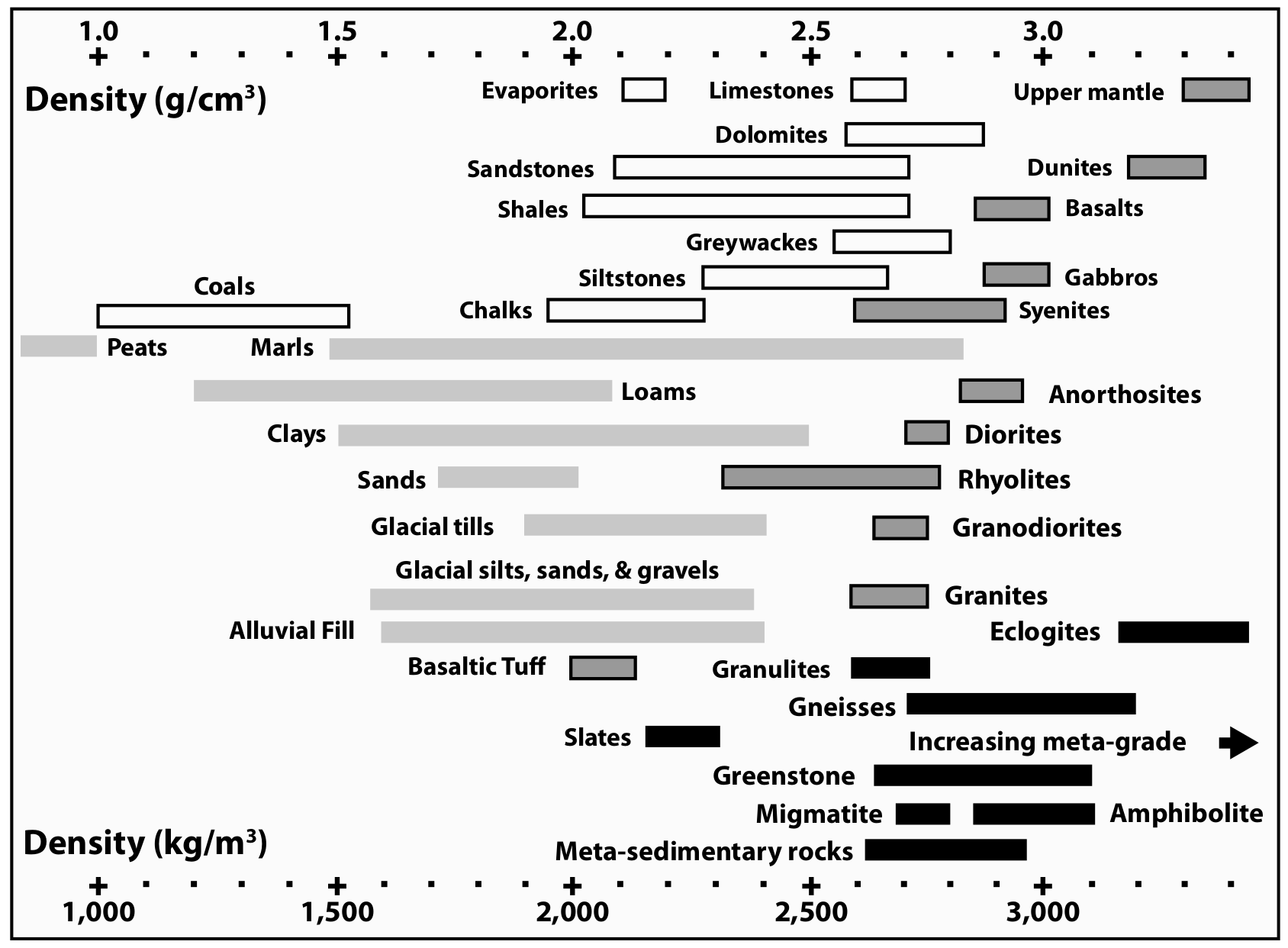
In the gravity survey, we use rock densities to identify rock types. Please select a density cutoff in each range (the blue boxes below) to identify rock types. Keep in mind that one box should not overlap many rock types or should cover a short range of rock types. Please select the best tree ranges.
cutoff 1
cutoff 2
cutoff 3
cutoff 4
cutoff 5
cutoff 6
cutoff 7
cutoff 8
cutoff 9
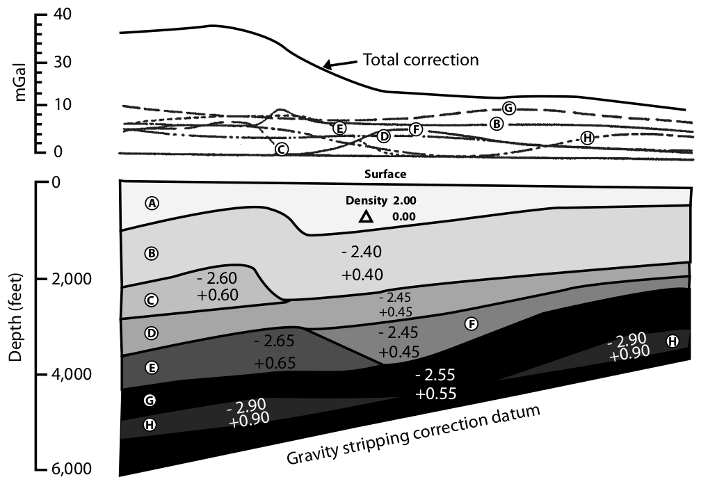
Gravity Correction
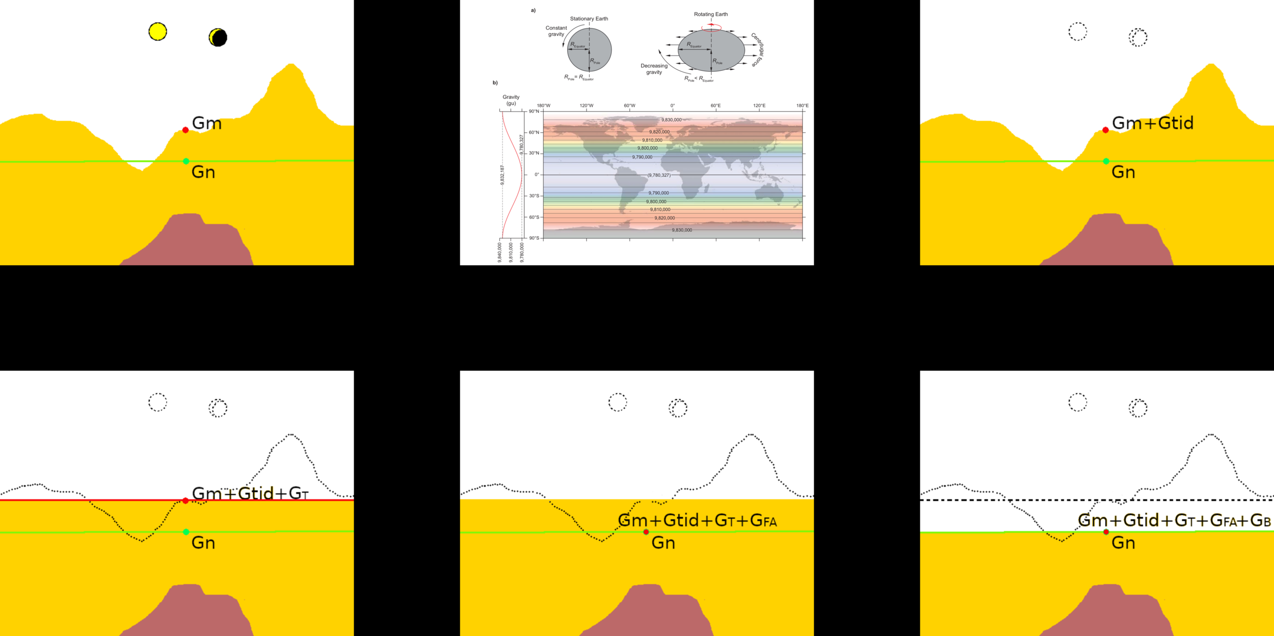
normal gravity
terrains
earth rotation
tides
free air
Bouguer
CH 3: Electrical Resistivity
Applications in Electrical Resistivity
Near-surface applications (less than 50 m), based conductive and resistive materials
-
groundwater aquifers
-
groundwater contamination
-
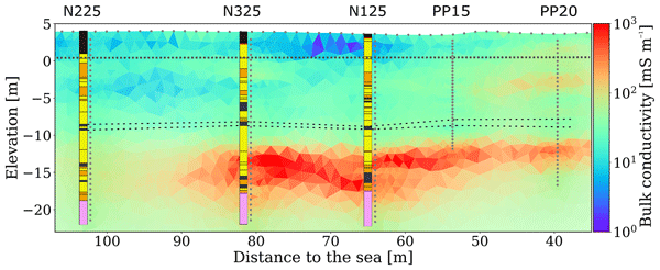
seawater intrusion
-
soil and bedrock detection
-
soil moisture
-
ores and mineral deposition
-
void and cavity detection
-
engineering construction detection
-
leak detection
-
agricultural monitoring
Direct Current (DC) Resistivity
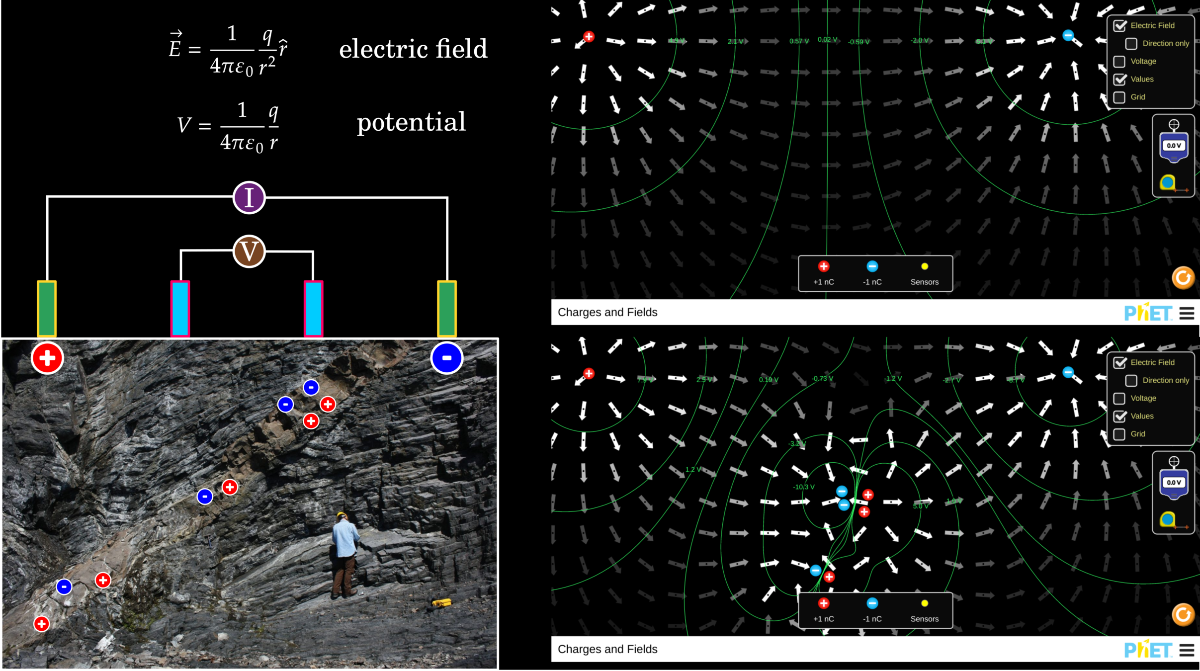
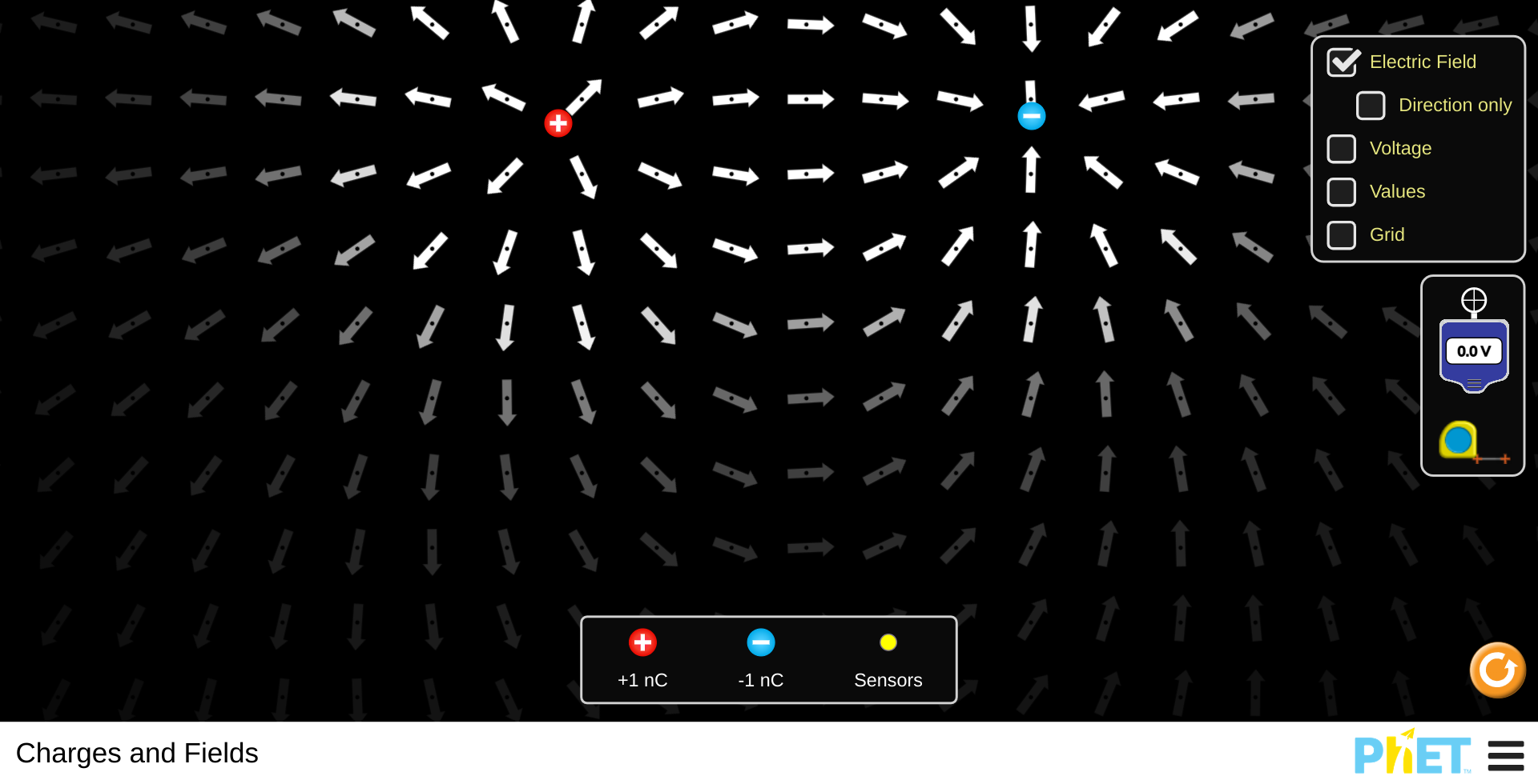
Gravity and Electric Fields
Text
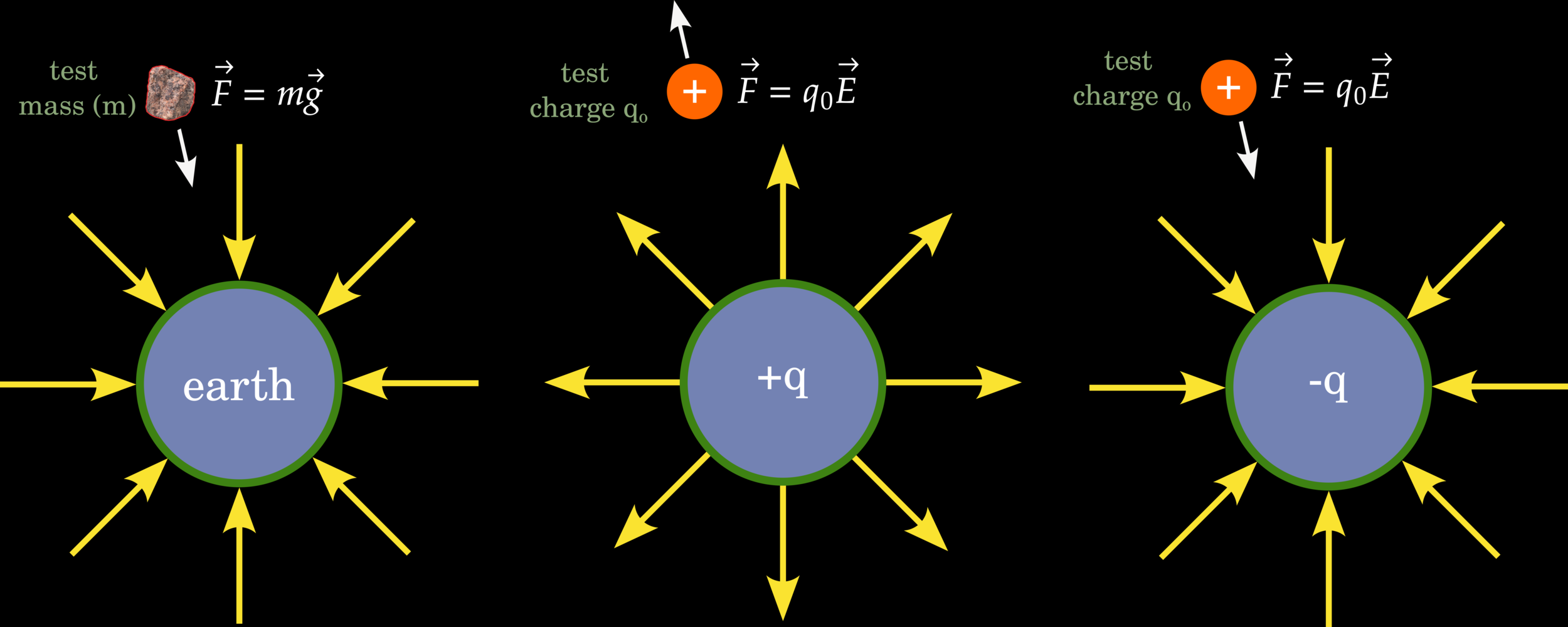
Electric Field Due to an Electric Dipole
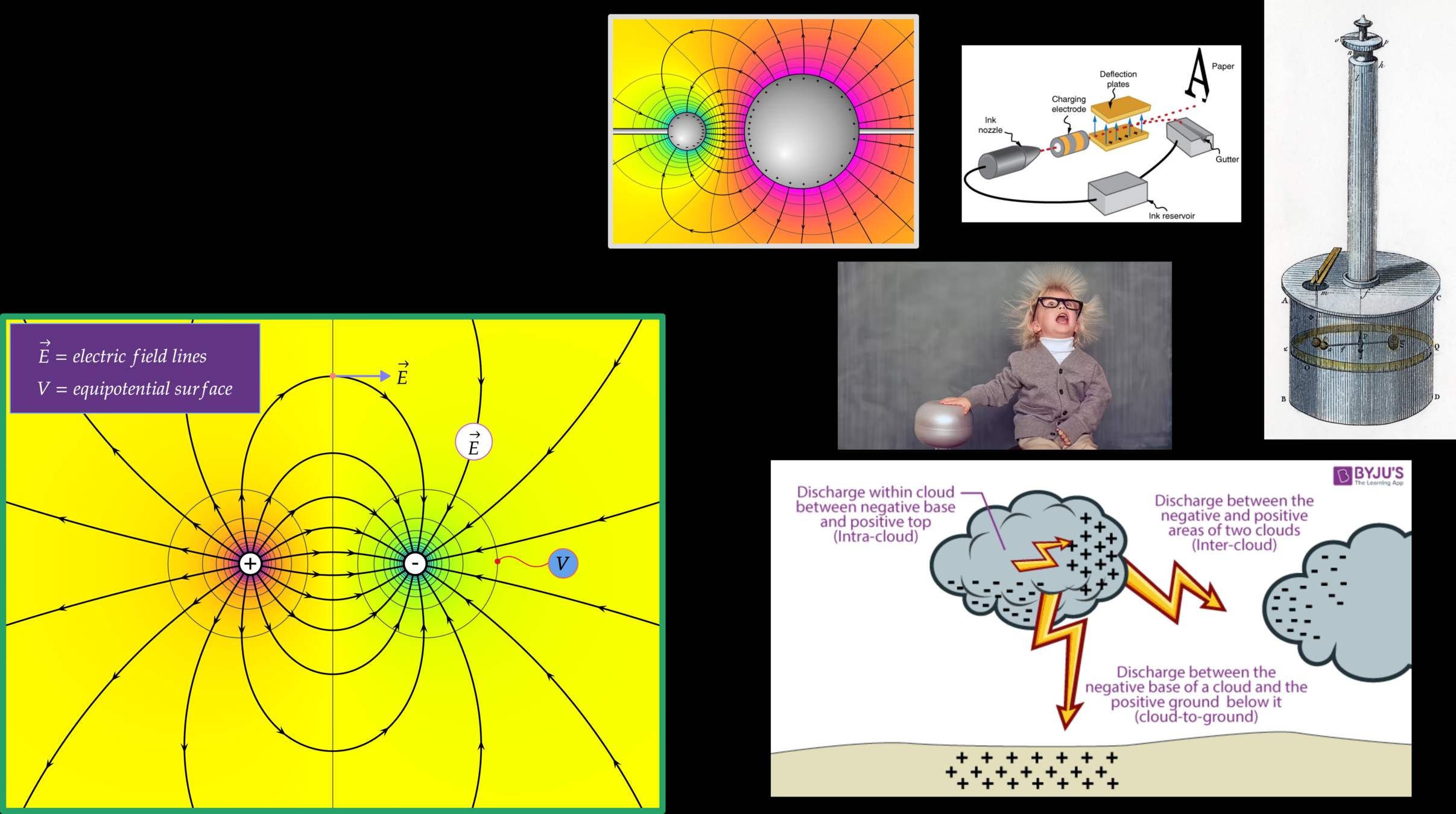
Coulomb's law
Takeaway Concept
DC Resistivity
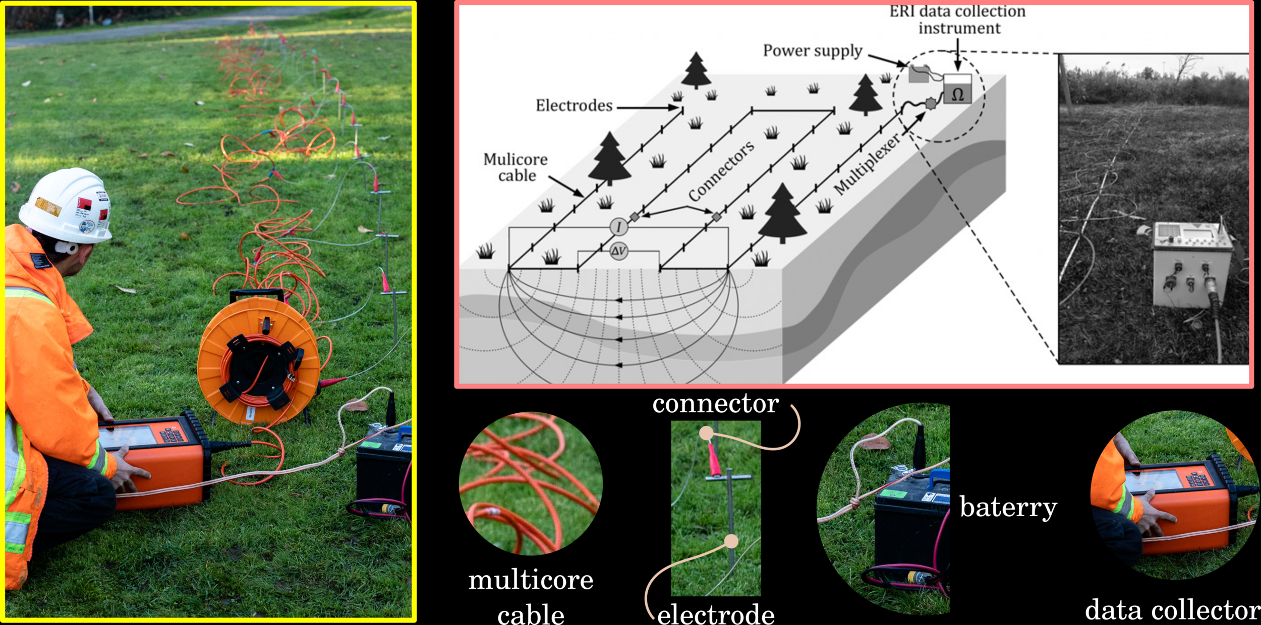
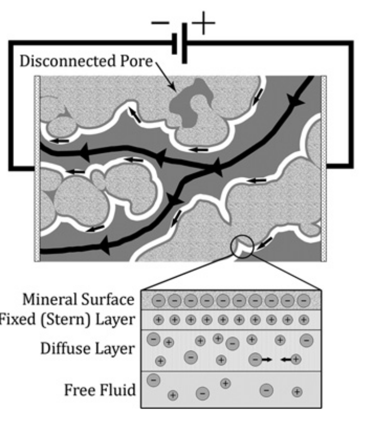
In this section we look at Direct Current (DC) resistivity surveys. The physical property of for DC surveys is electrical conductivity σ (Siemens/meter) (or if you prefer its inverse, resistivity ρ (Ohm * meter)). For these surveys, the source is current injected into the ground, and the receivers measure the strength of the current and voltage differences.
DC resistivity is widely used for mining exploration, particularly for porphyry deposit, in geotechnics to find cavities in the subsurface or in environment to determine possible pollution leakage.
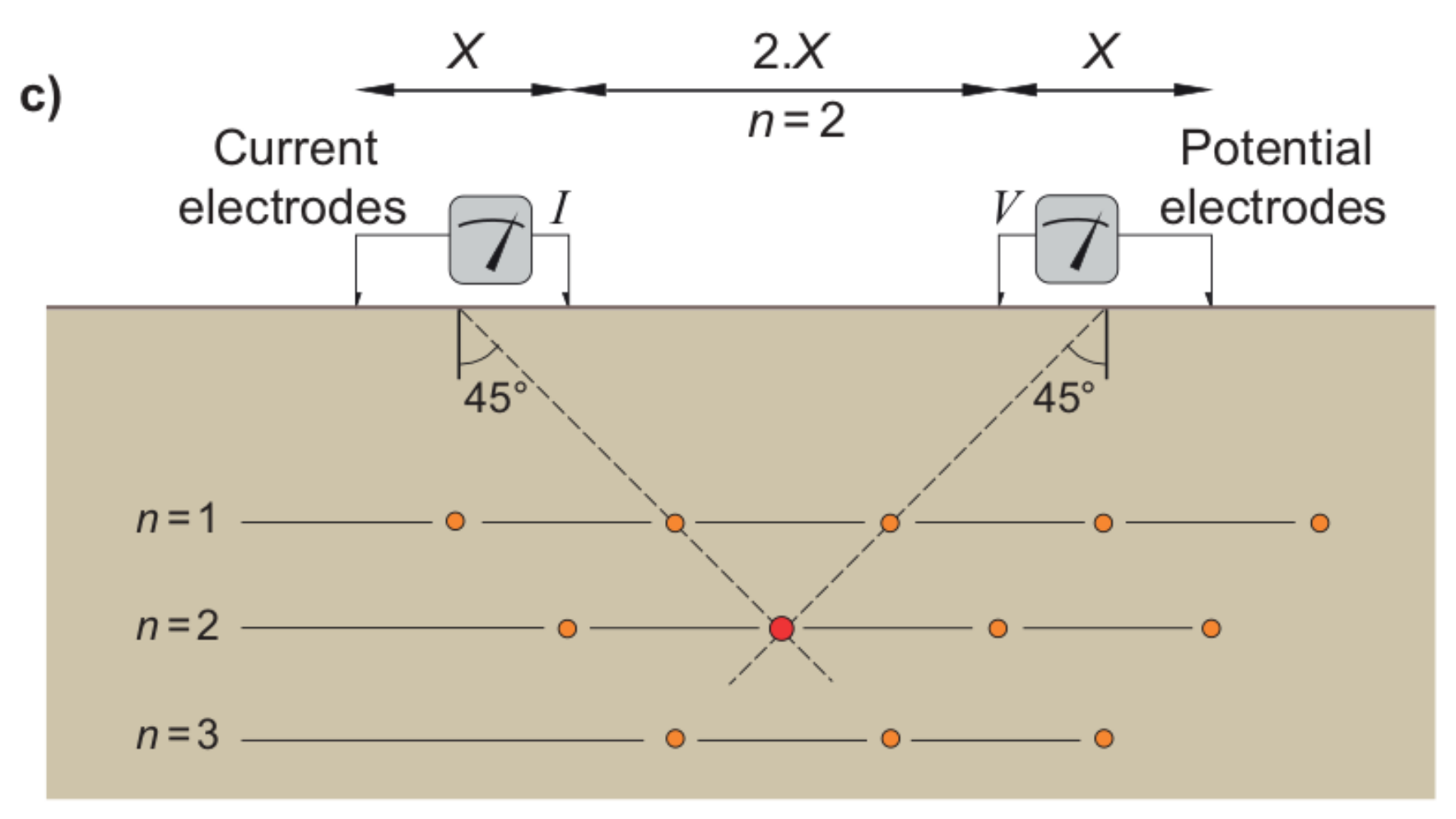
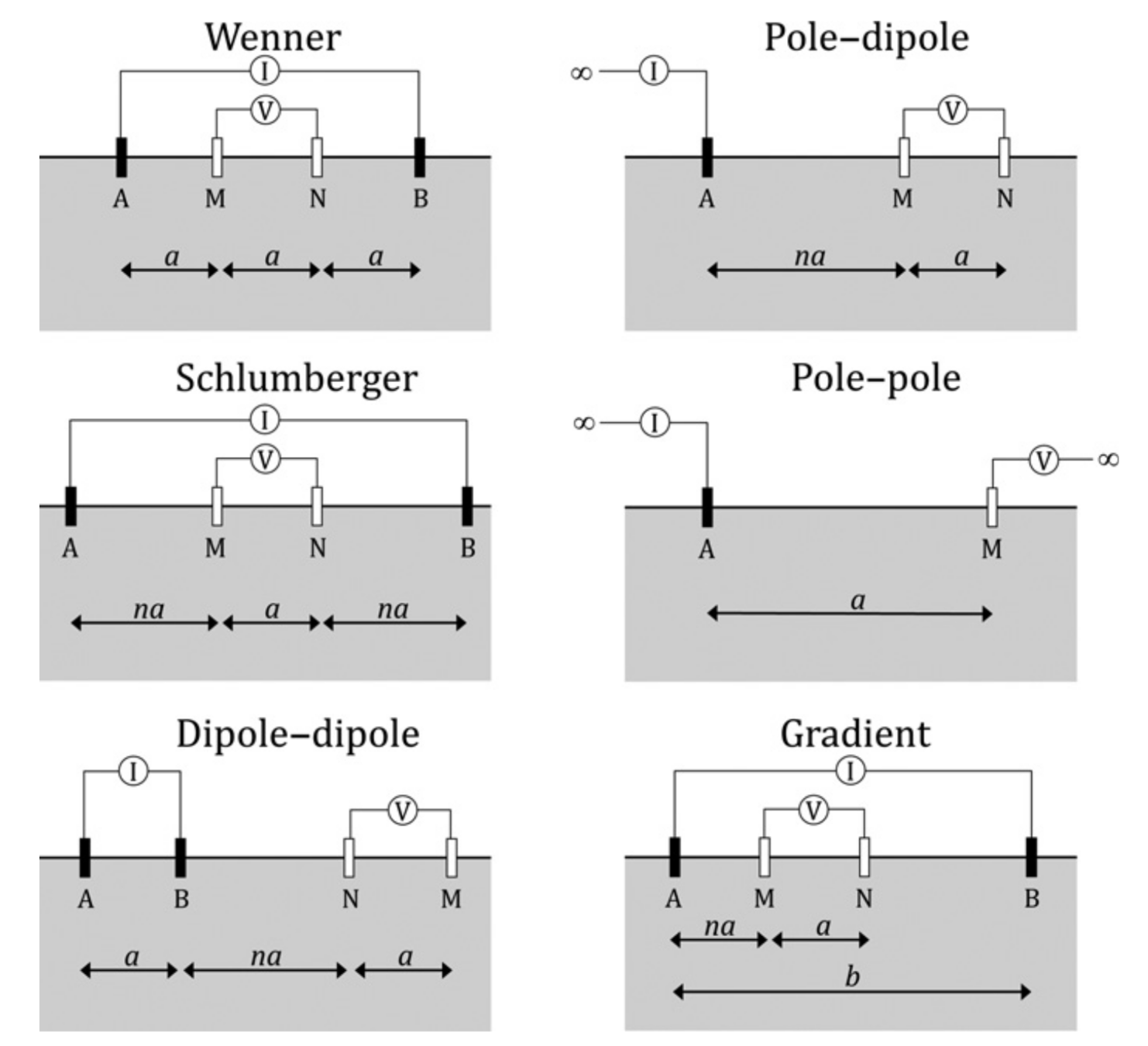
Some key areas to pay attention to with DC surveys are the various configurations (dipole-dipole, pole-dipole, gradient array, Schumberger and Wenner soundings), each of which delivers a particular focus on different subsurface information.
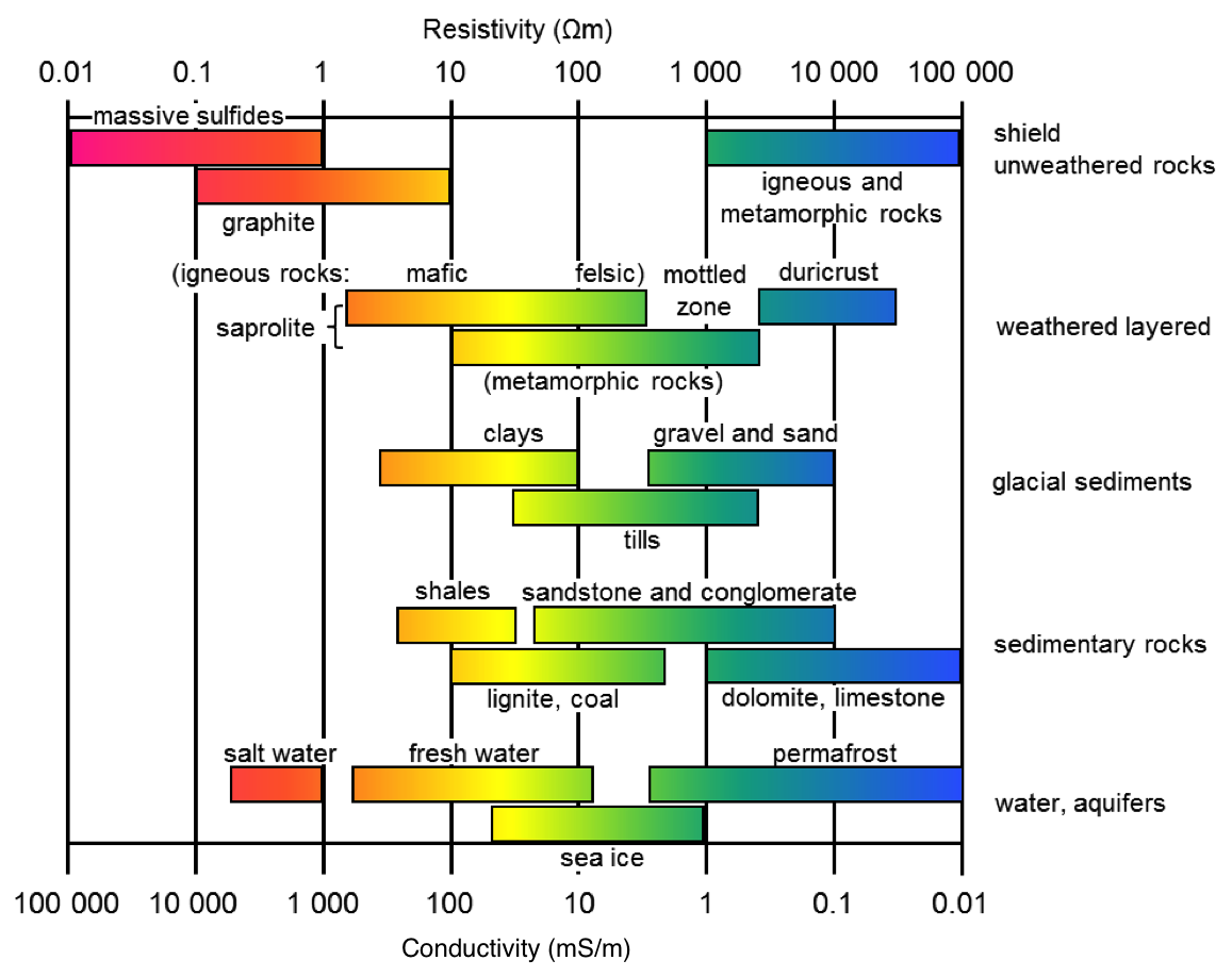
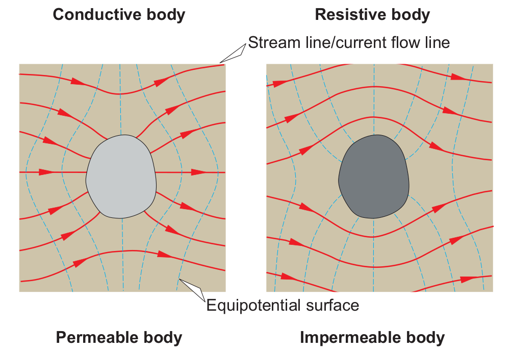
conductivity and resistivity
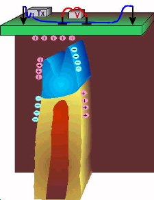
Two electrode current sources
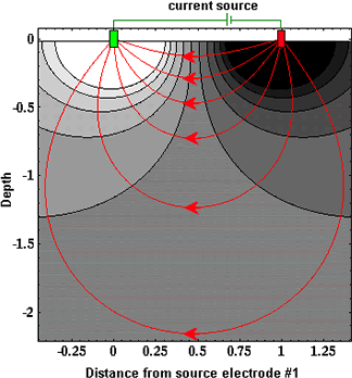
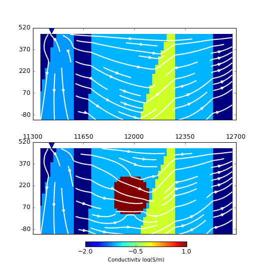
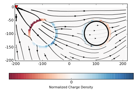
Currents and Voltages in an Heterogeneous Earth


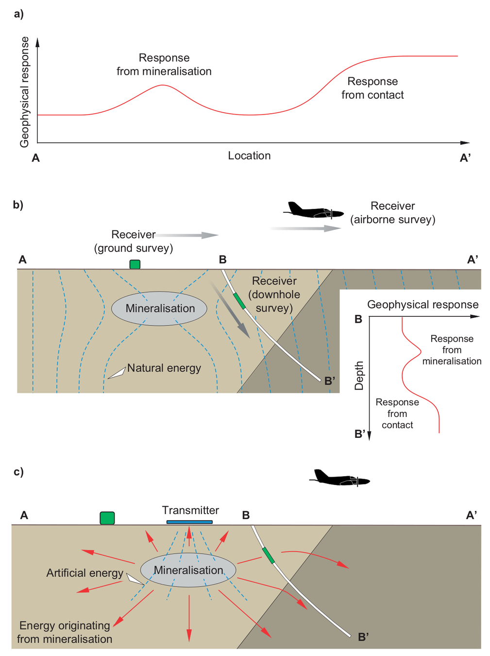
Surveys
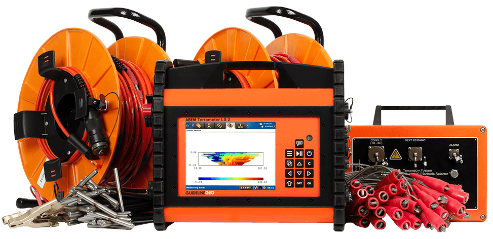
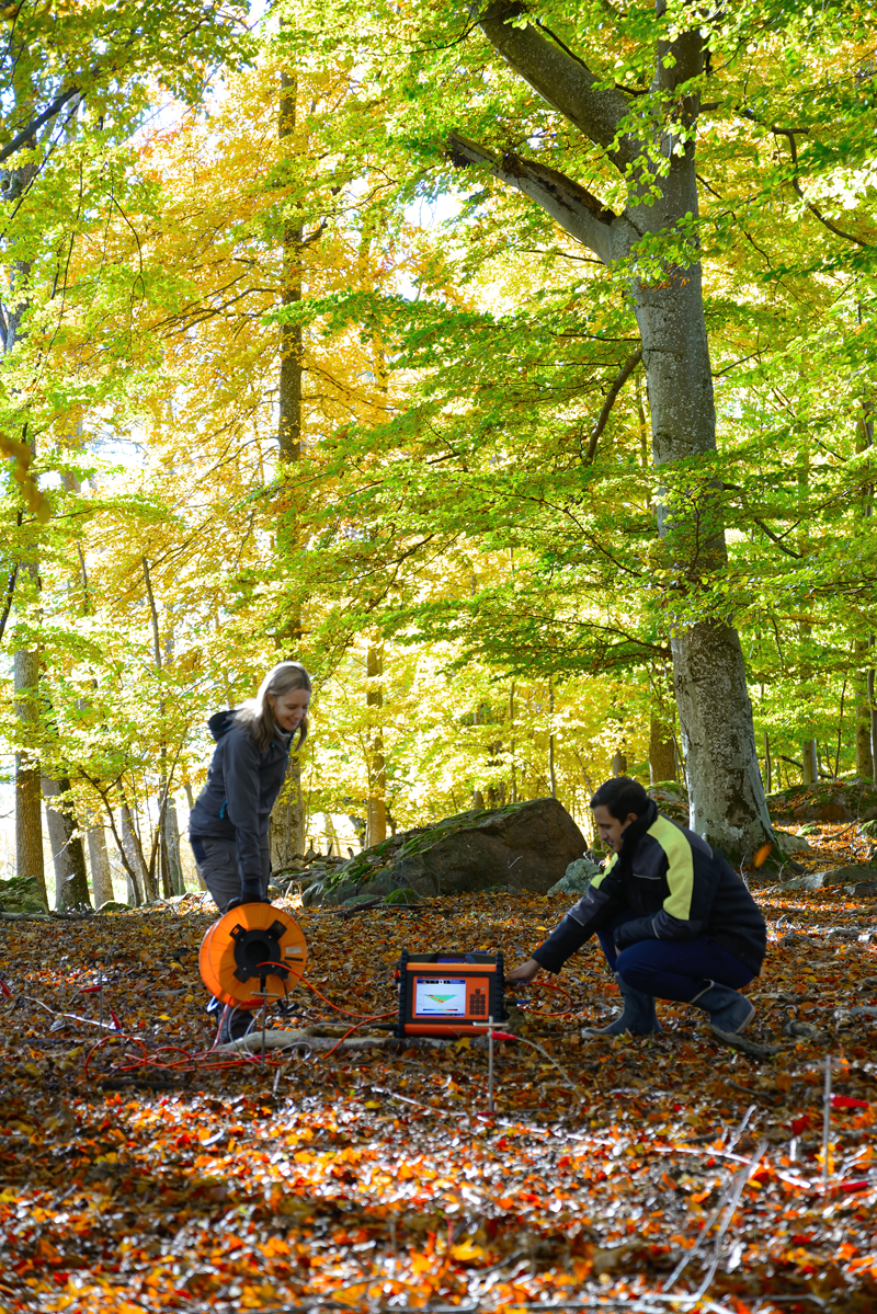
High power and reliable constant current are the primary requirements of DC resistivity transmitters. For small scale work (electrodes up to roughly 100 m apart), a transmitter capable of sourcing up to several hundred milliwatts of power might be adequate. For larger scale work (electrodes as much as 1000 m or more apart), it is possible to obtain transmitters that can source up to 30,000 watts. See the section DC resistivity instruments for more details.
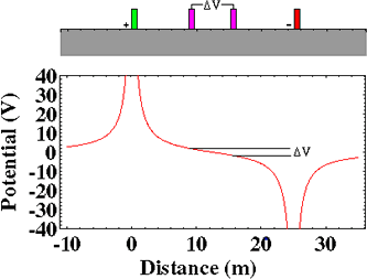
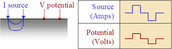
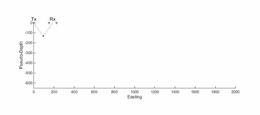
Source (Tx)
Measurements (Rx):
potential difference
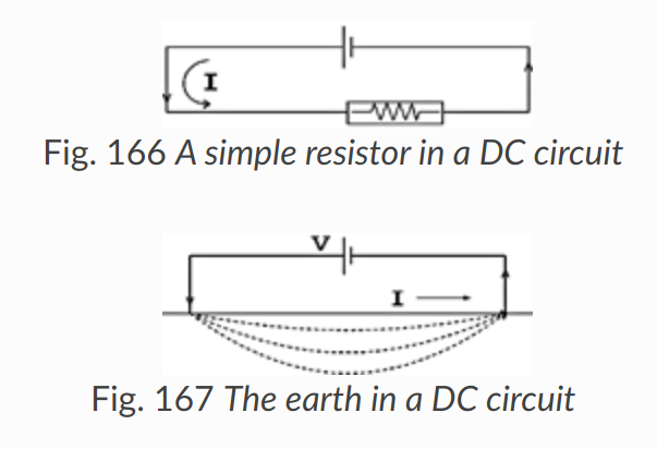
It is tempting to compare the earth to a resistor in an electric circuit (Fig. 166, Fig. 167). However, it is important to recognize the difference between resistance and resistivity. If we apply Ohm’s law, R=V/I we will have a resistance, which is in units of Ohms. This is not the ground’s resistivity, which has units of Ohm-m. We do not want the resistance of this circuit, we want a measure of the ground’s resistivity.
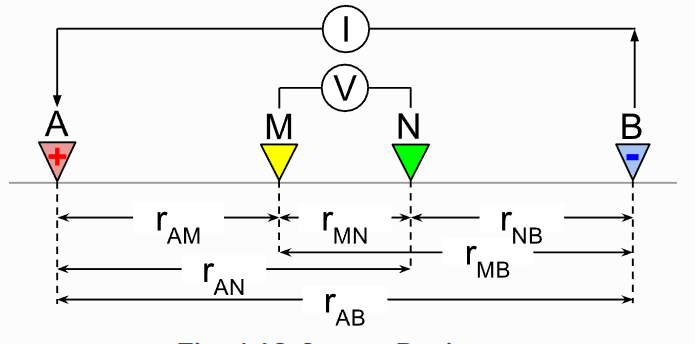
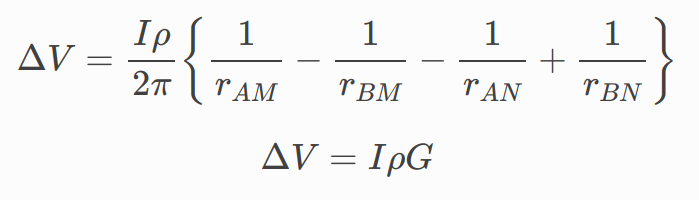
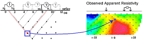
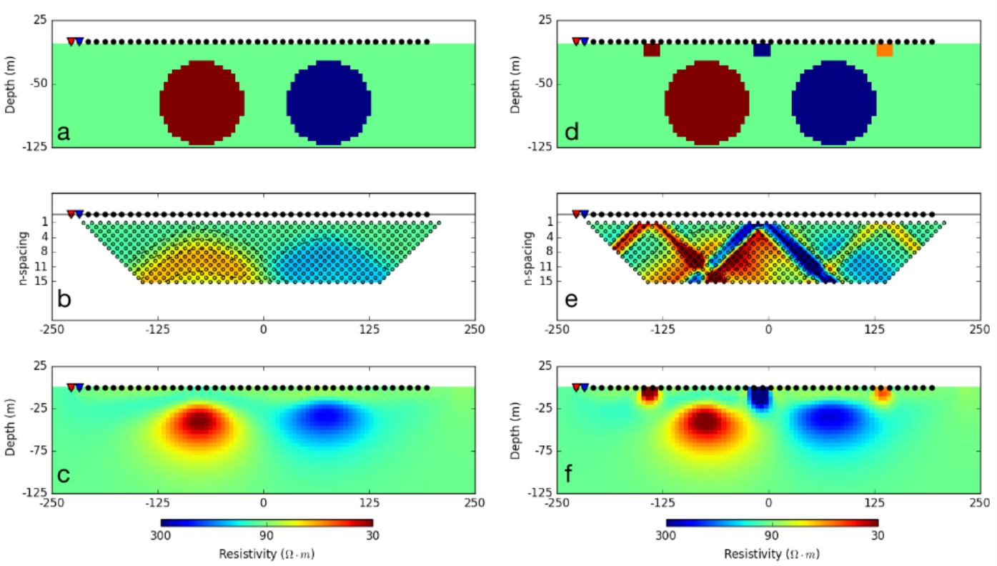
Measurement configuration
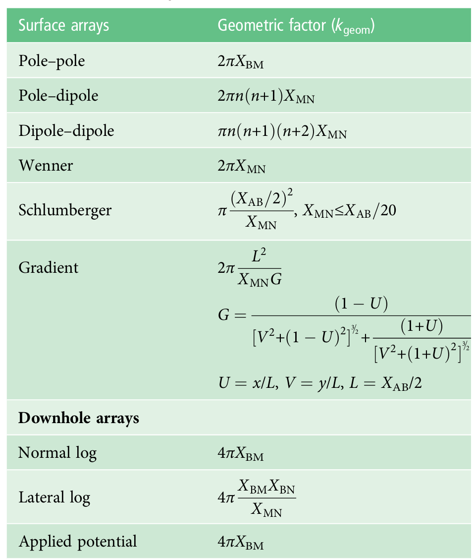
DC Resistivity Arrays
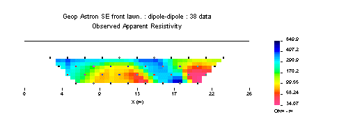
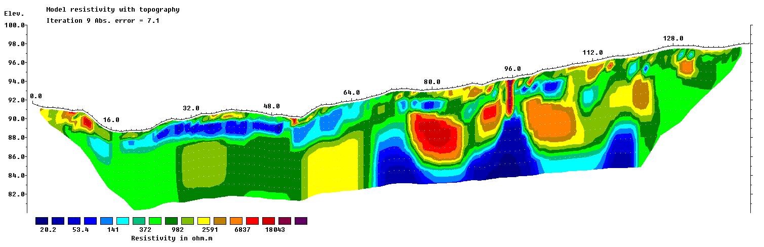
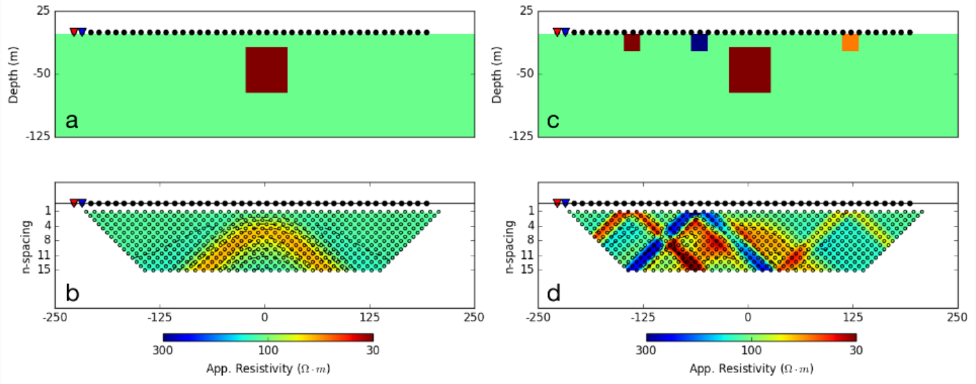
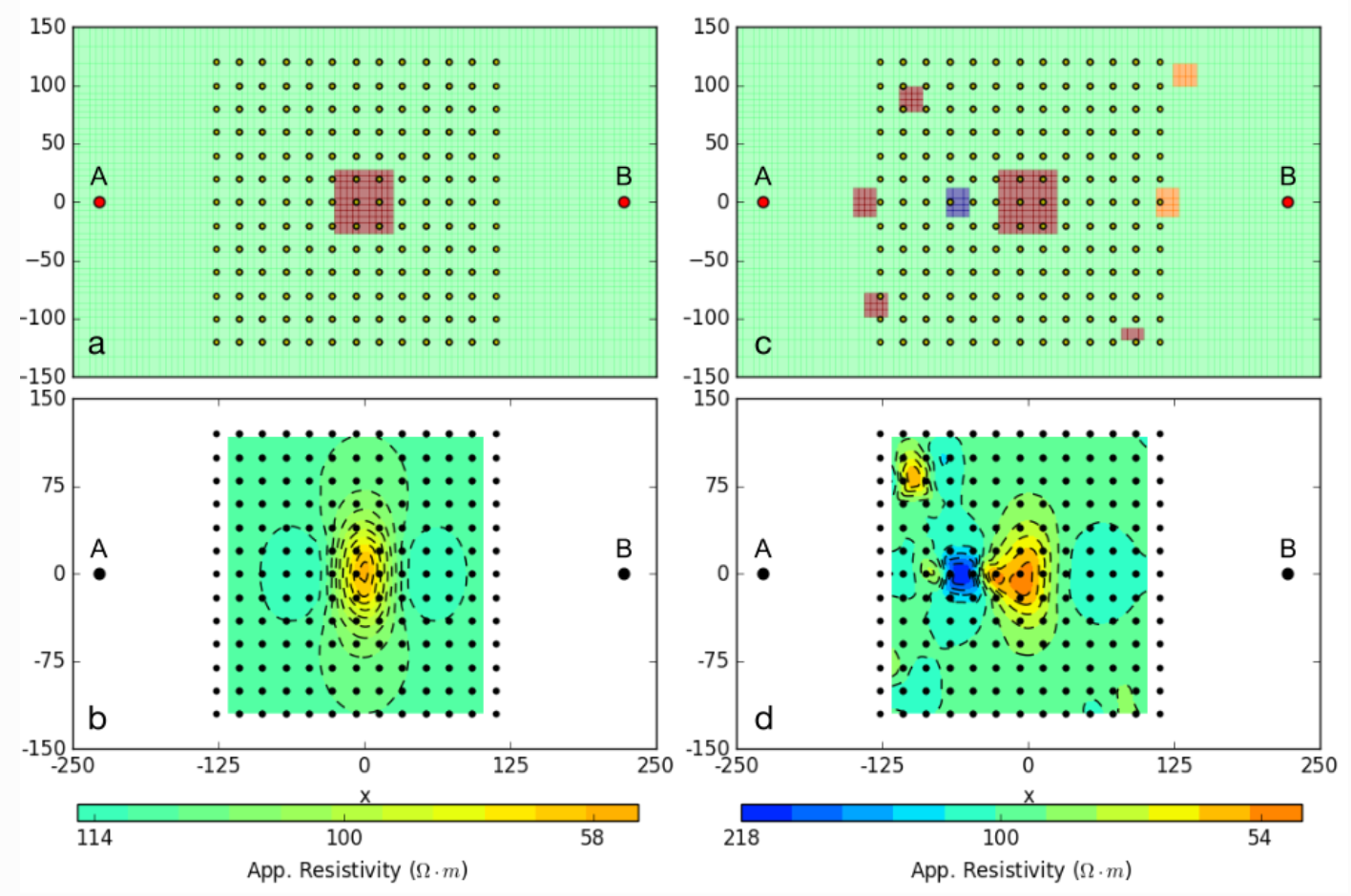
Interpretation
Midterm Score

CH 4: Seismic
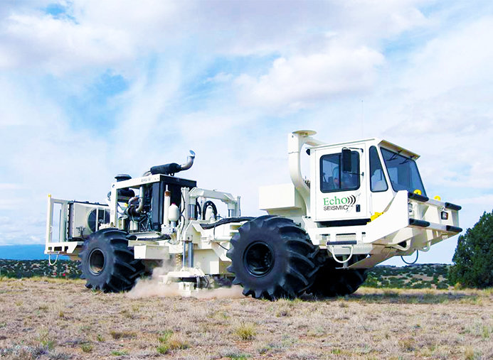
Seismic Exploration
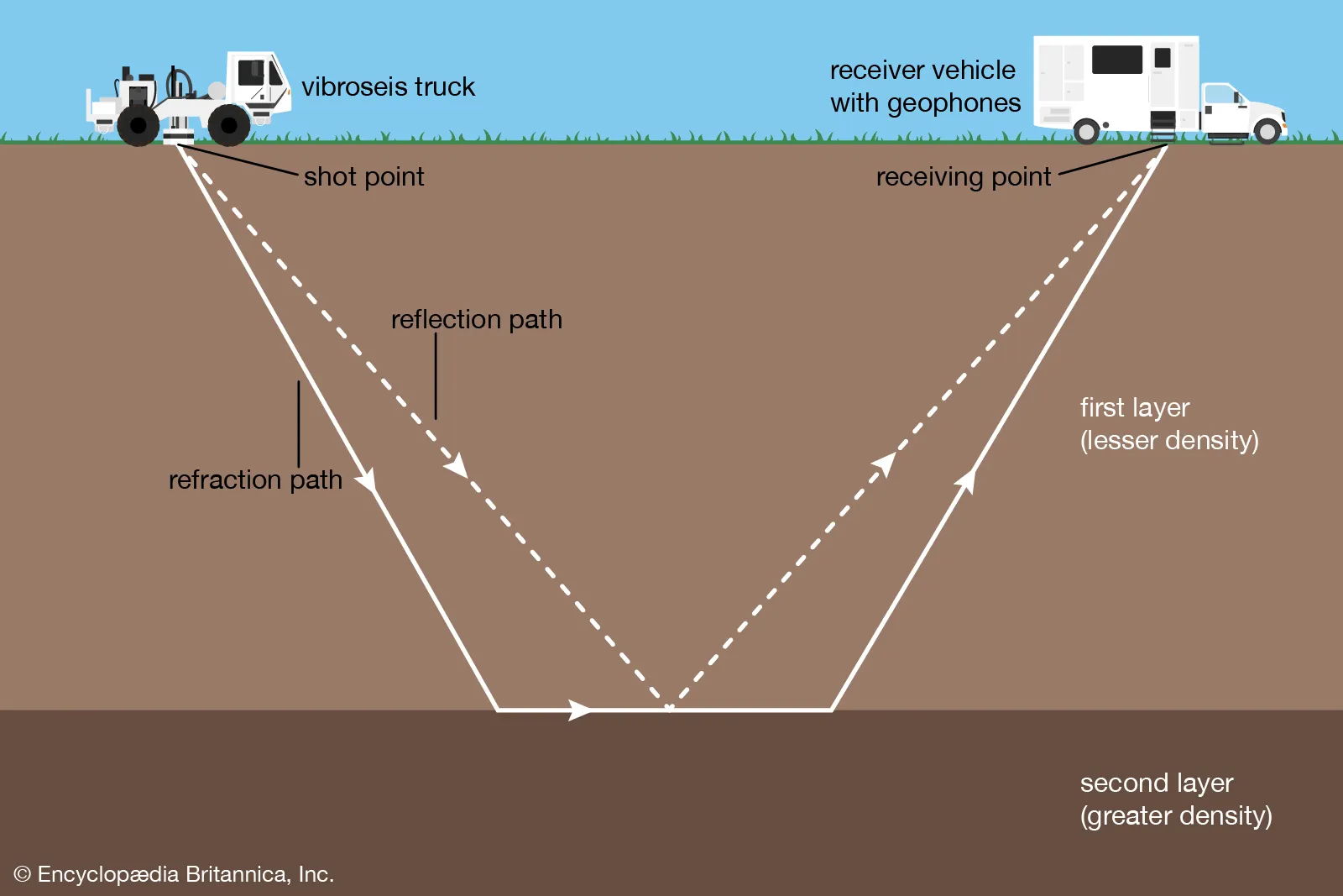
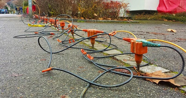
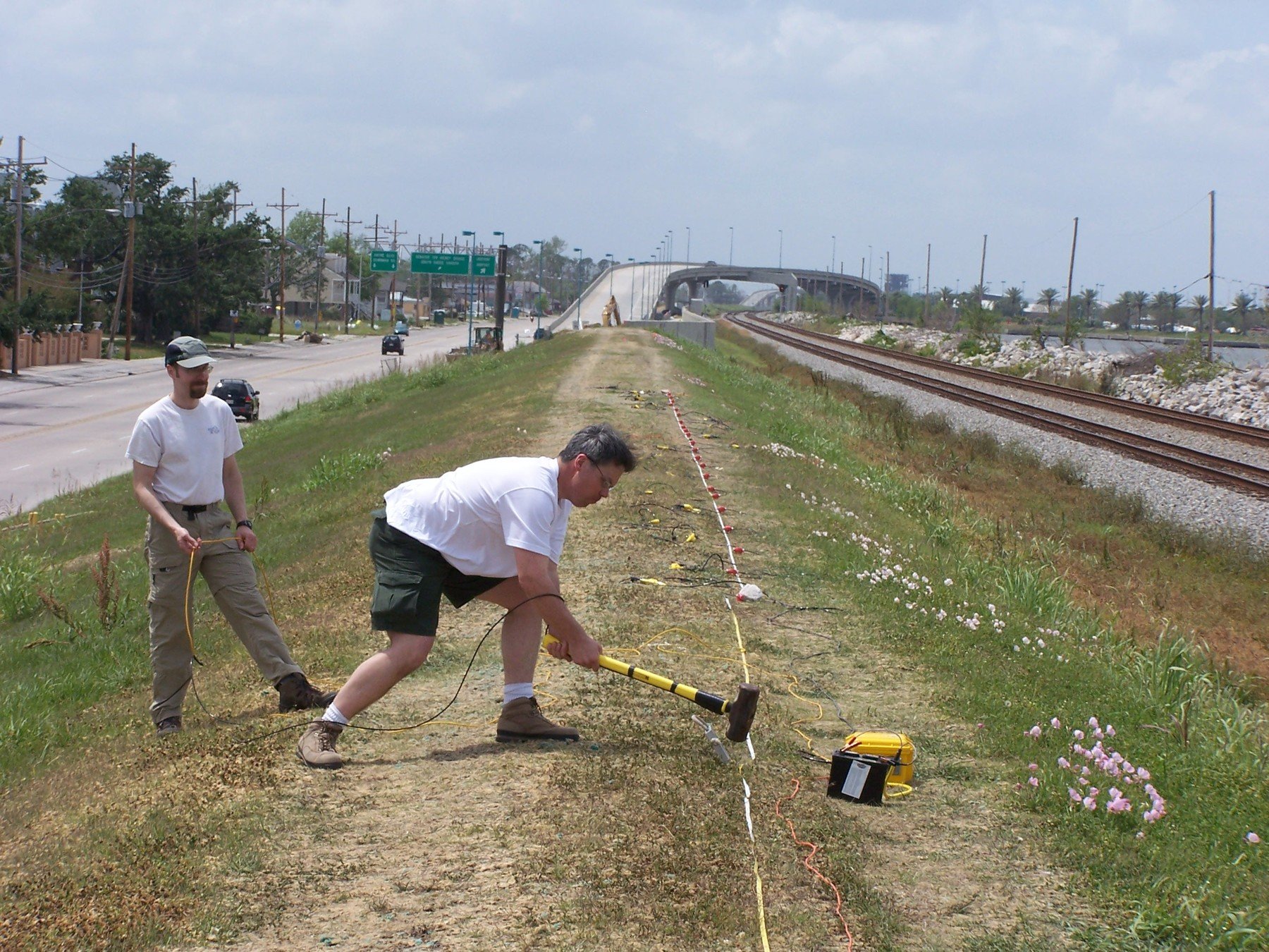
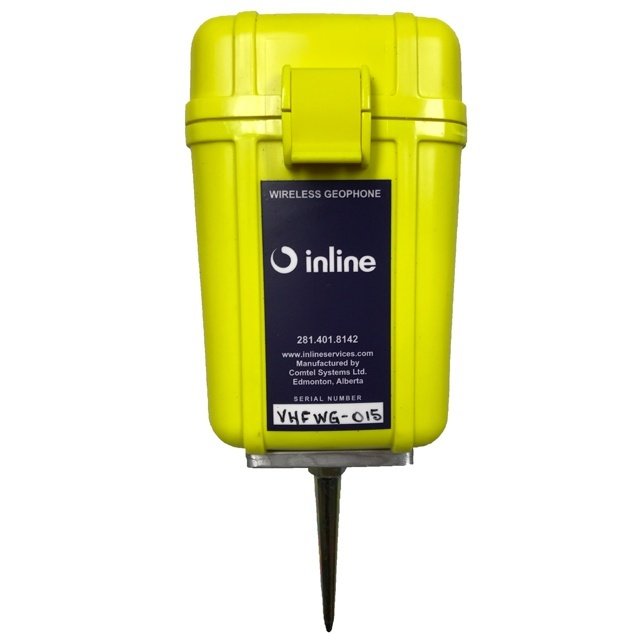
Source and Recivers
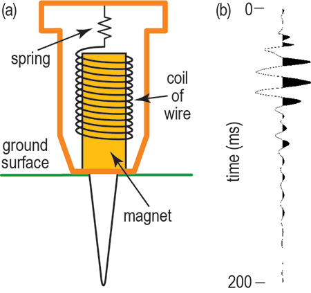
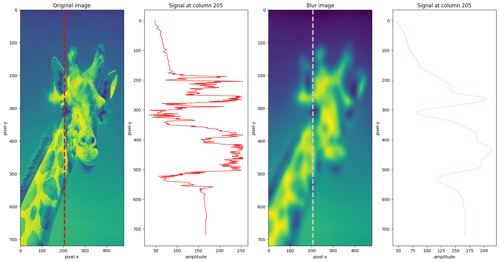
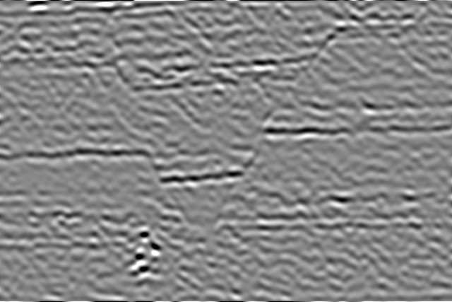
Seismic Image
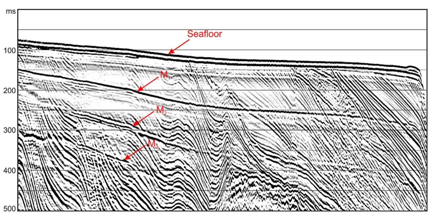
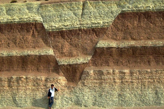
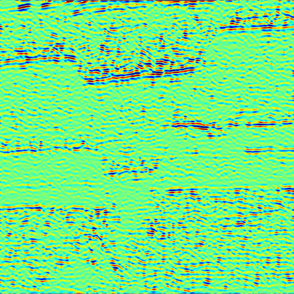
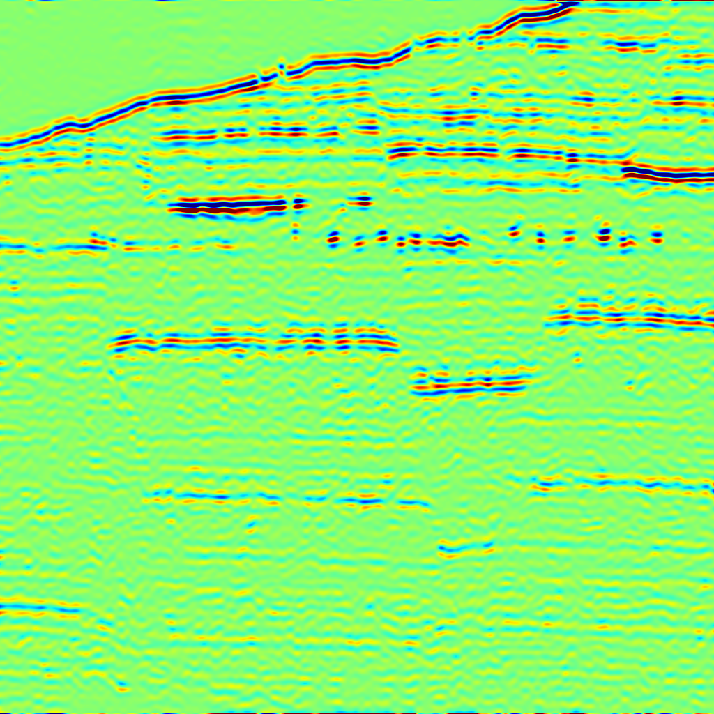
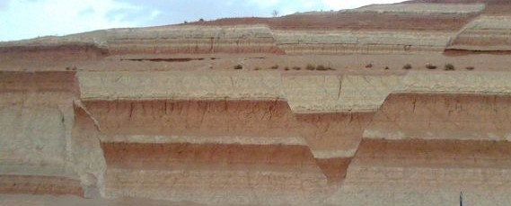
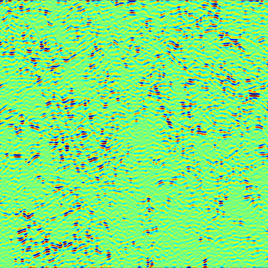
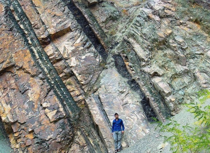
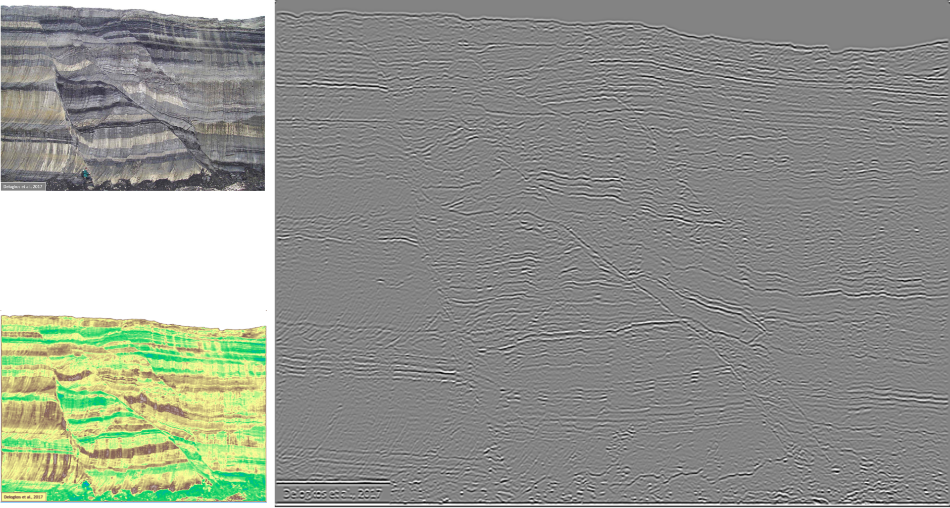
Before going straight into seismic imaging theory, let us have a glimpse of seismic images. The outcrop image is on the top left, and the seismic image is on the bottom left. The seismic wave can capture just some frequency range in which most outcrop details are partially preserved.
The signal at the location (inline 205) is an example of a 1D signal that contains different dominant frequencies: the outcrop image contains a higher.

Simple Harmonic
1 hertz = 1 Hz = 1 oscillation per second = 1 s
-1
T = \frac 1 f
2\lambda = T
amplitude
phase\ angle\ \theta\ =\ 0
Use the Harmonic equation to reproduce the cosine function shown in the figure above. Try to modify the parameters such as amplitude, frequency, and phase. You might superimpose your results to analyze what differences are.
Simple Harmonic Superposition

What Is the Composition of This Waveform?

Almost waveforms in seismic exploration combine various sine and cosine functions, amplitudes, and phases. It is rare to find a simple harmonic form. Generally, geophysicists approximate seismic frequency as an average frequency, and this estimation refers to the dominant frequency, many frequencies, but a few frequency ranges dominate the spectrum.
Can we generate some sine and cosine functions to fit this waveform?
Fourier Series


Using the Fourier series, the equation above generates several sine and cosine functions and sums all functions together. We notice that the coefficients can expand by using Euler's formula.
The Figure on the left represents the number of generated functions from sines and cosines. Theoretically, the integration form should reach infinity to generate a fit function. Here, we approximate only five times and yield a decent fit function.
true signal
Discrete Fourier Transform


Fourier transform integral

Fourier inversion integral
Excerise
Use DFT to compute the frequency at the window. The approximation is based on the summation of the vertical signal in 1D.
Wave Equation
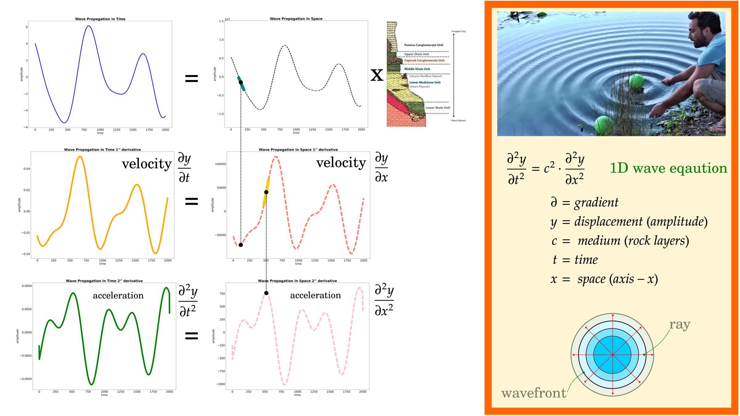
What is "c" in Wave Eqaution

Beyond Acoustic Wave: Elastic Wave
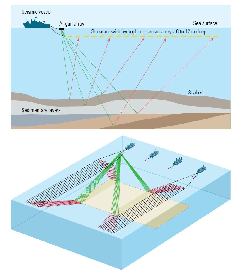
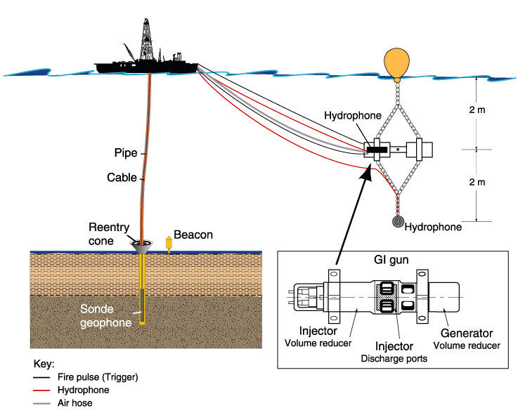
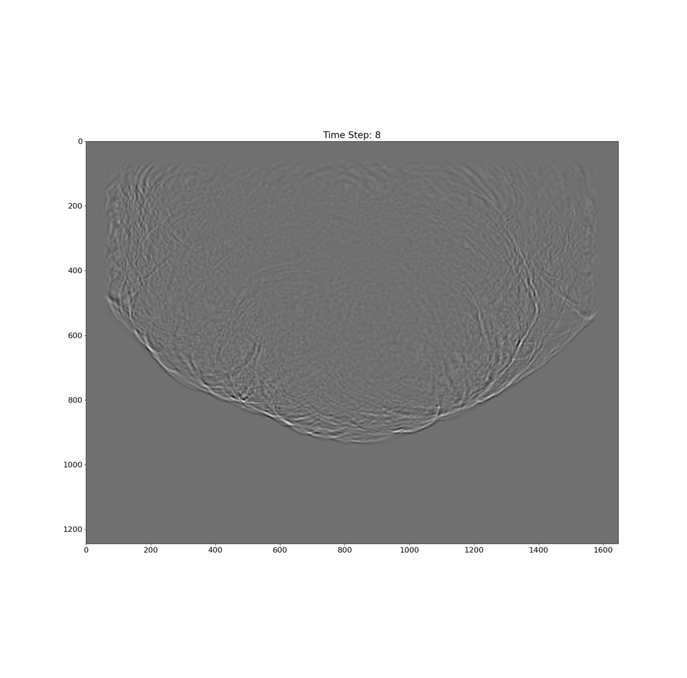
Wave Propagation in Seismic Exploration
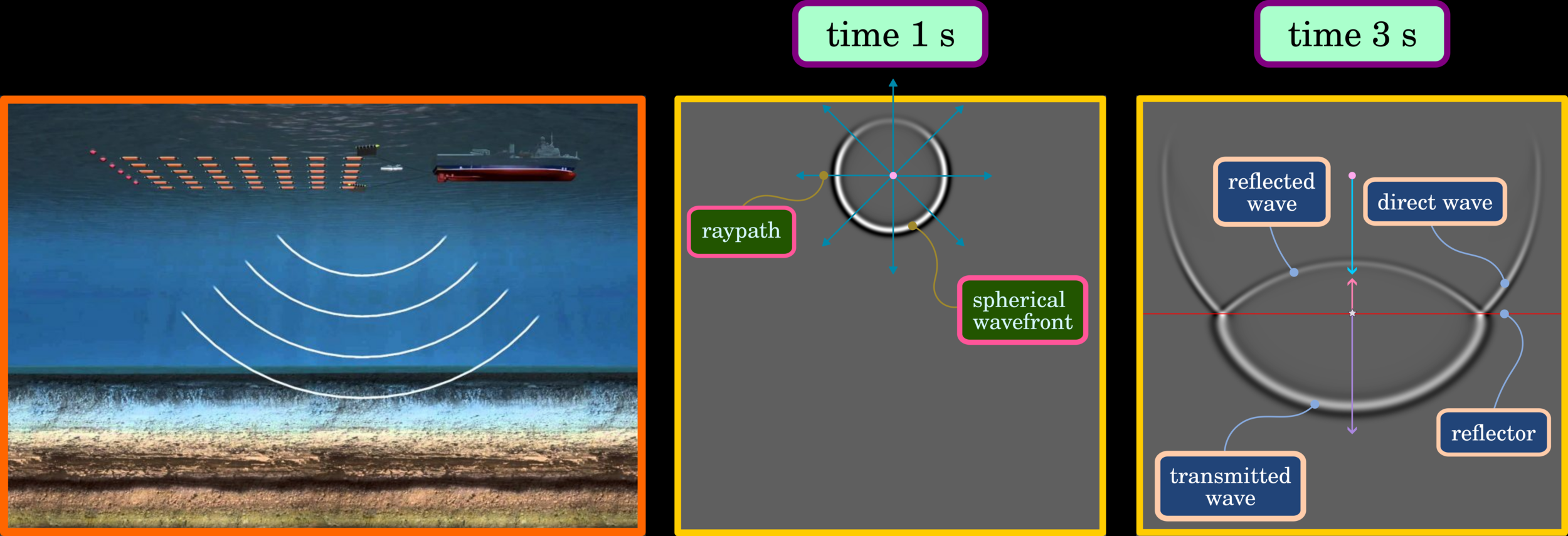
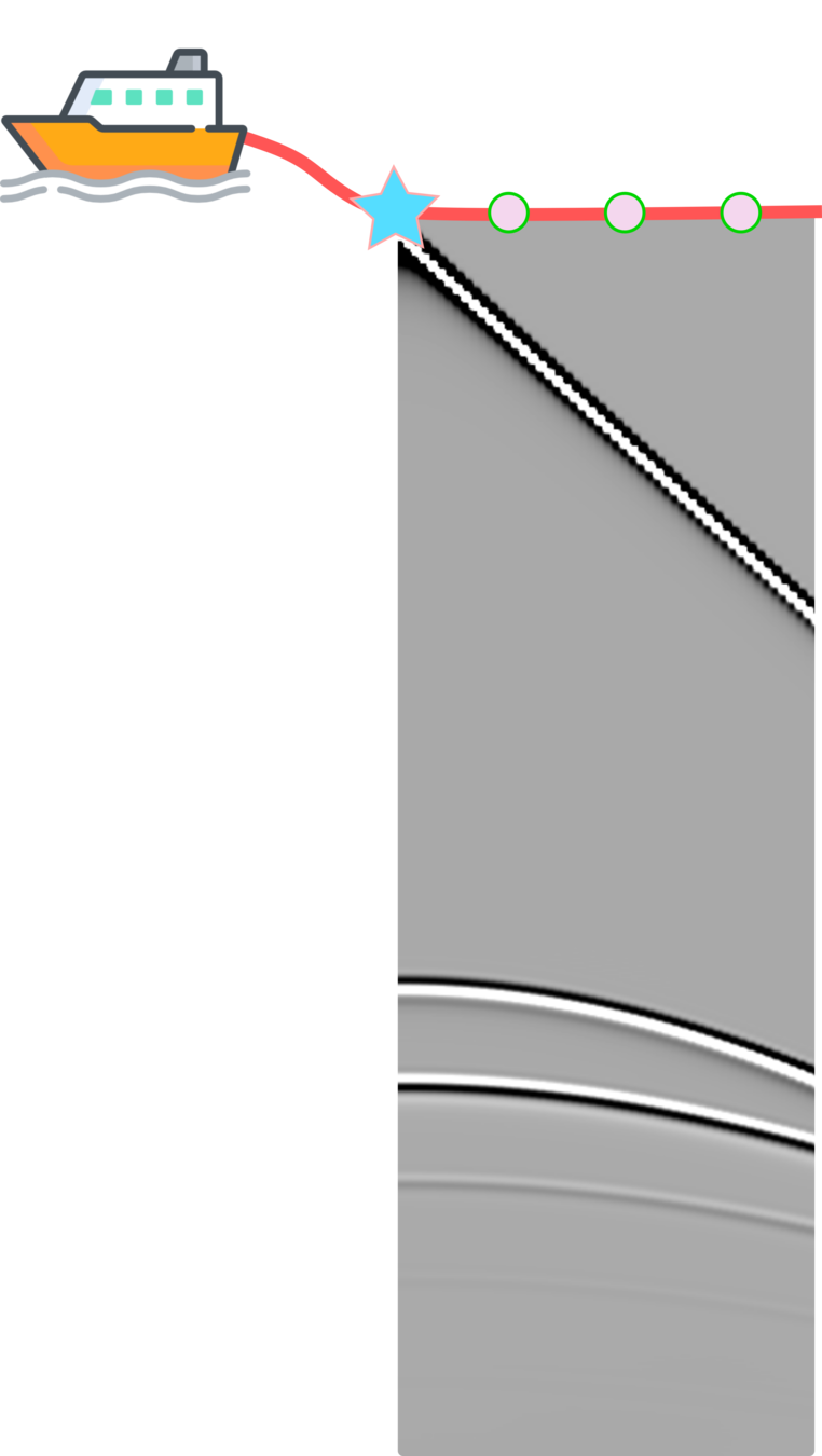
Wave propagation in exploration refers to exploding energy from a source, in this case using an airgun, and wave propagates in all directions, such as the figure in the middle. The wave propagates through the medium, that is, seawater and rock under the sea floor. Once the wave hits the reflector (sea floor), it will partially reflect, returning to the surface and partially transmitted through the subsurface. These wave phenomena are the principle of seismic exploration used for imaging subsurface.

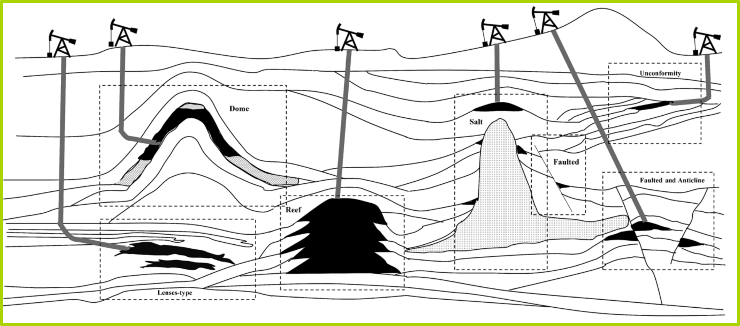
In the past, petroleum systems were likely uncomplicated structures. Nowadays, remaining hydrocarbon accumulations have more challenging structures requiring advanced geophysics methods to reveal a prospective target.
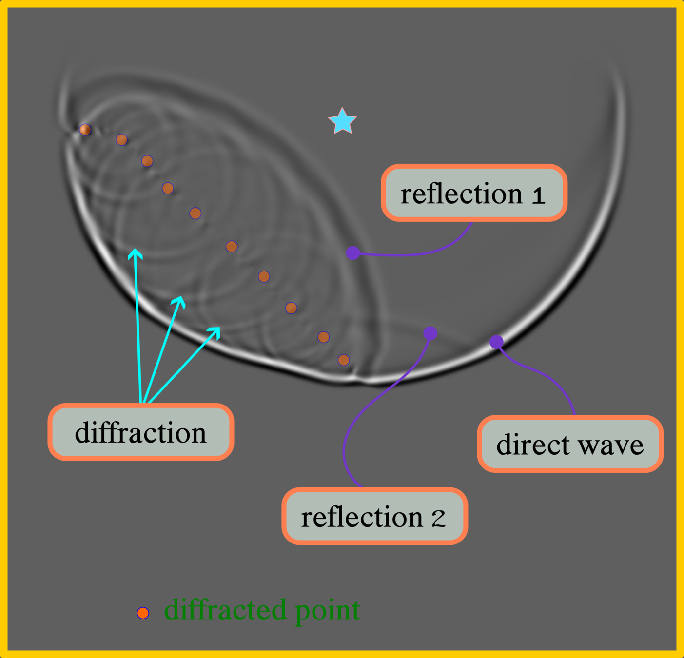
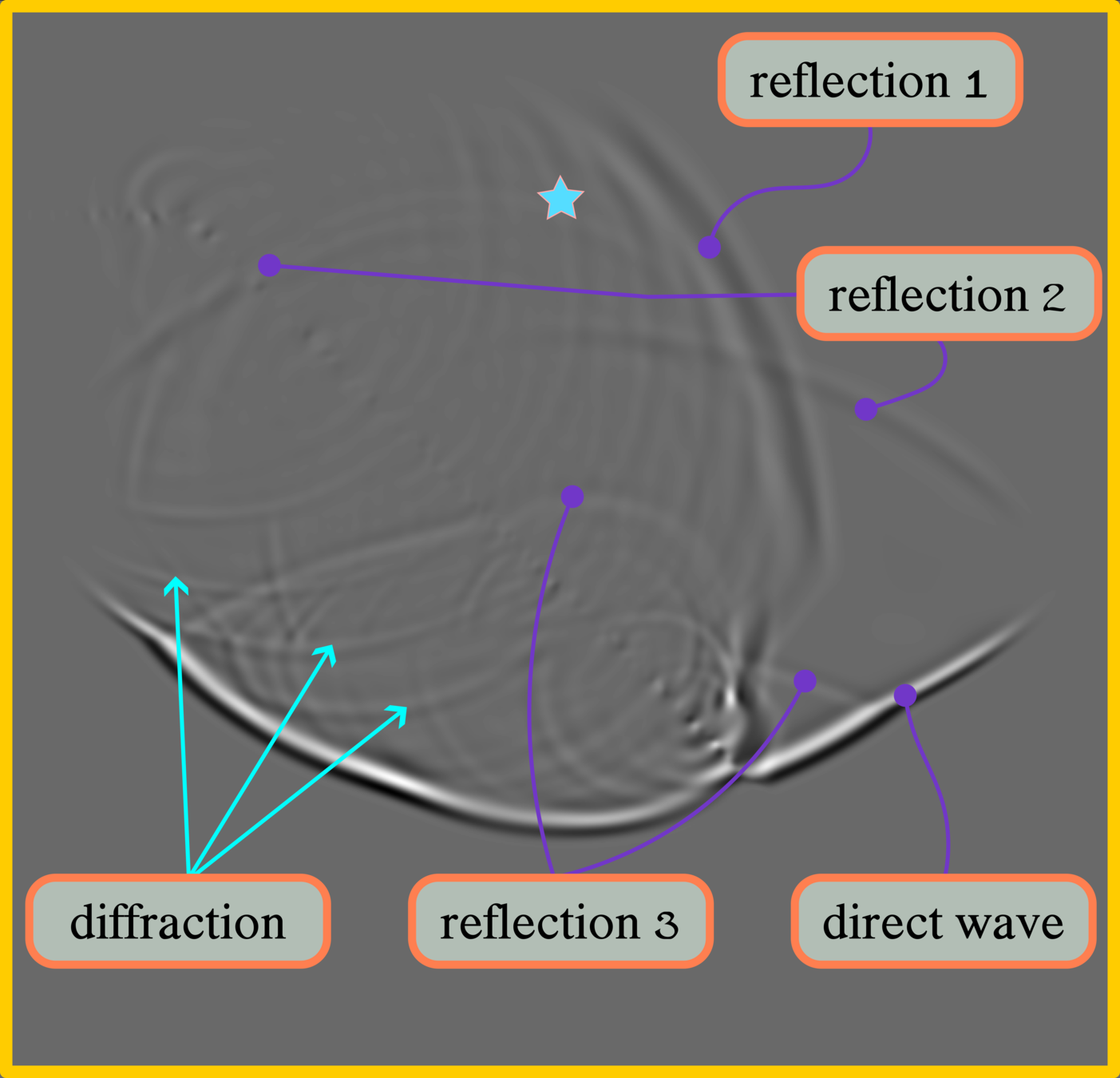
Diffraction
The Huygens–Fresnel principle (named after Dutch physicist Christiaan Huygens and French physicist Augustin-Jean Fresnel) states that every point on a wavefront is itself the source of spherical wavelets, and the secondary wavelets emanating from different points mutually interfere.[1] The sum of these spherical wavelets forms a new wavefront. As such, the Huygens-Fresnel principle is a method of analysis applied to problems of luminous wave propagation both in the far-field limit and in near-field diffraction as well as reflection.


diffracted point
Diffraction
The reconstruction of seismic images is based on scattering theory, which can explain by diffraction. When we solve a computer's continuous wave equation with limited memory capacity, we assume that each element in computer memory can generate the seismic wave, called the point source. If several point sources have wavefronts superposition strong enough, this phenomenon can form seismic reflection. So both terms share an essential relationship.
diffraction 1 point
diffraction 4 points
reflection


diffraction point
diffraction hyperbola

diffraction hyperbola
diffraction point

multi-diffraction points
reflection hyperbola
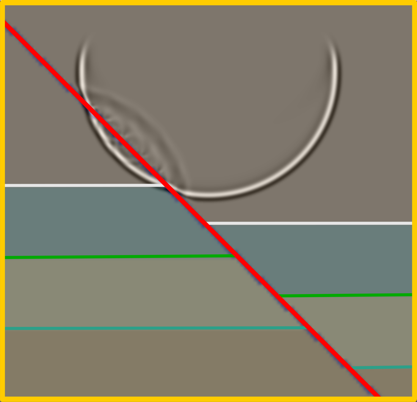
Wave Propagation in Geological Structure

model
time step
17
time step
21
time step
27
time step
37
This geological structure shows the normal fault that creates foot (left) and hanging (right) walls. The fault in this model represents sediment filled that creates a particular P-wave velocity zone. Three-layer sediments contain different P-wave velocities, and their quantitative information can refer to the code in our repository on GitHub. For simplicity, the model contains only P-wave velocity.
Wave Propagation in Geological Structure

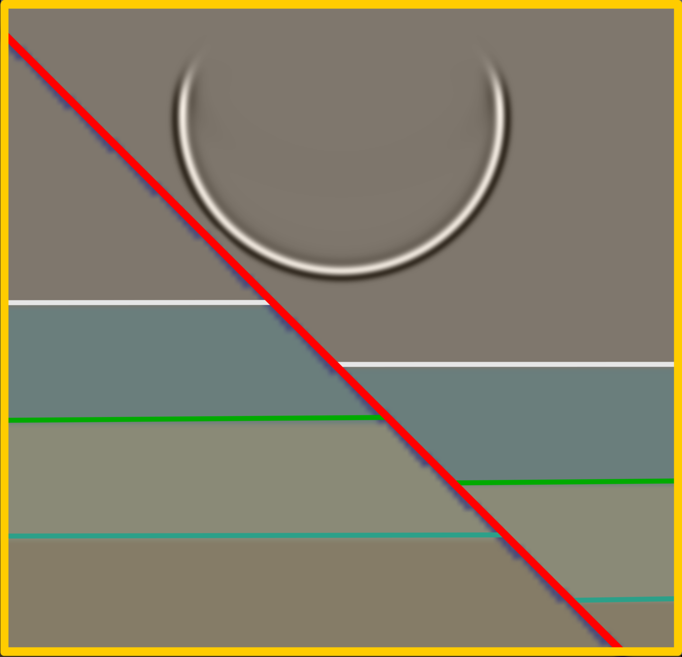
model
time step
17
time step
21
time step
27
time step
37
The direct wave indicates the sound wave spreading as a spherical wave. In a homogeneous medium, the spherical wave will maintain its symmetrical spreading.
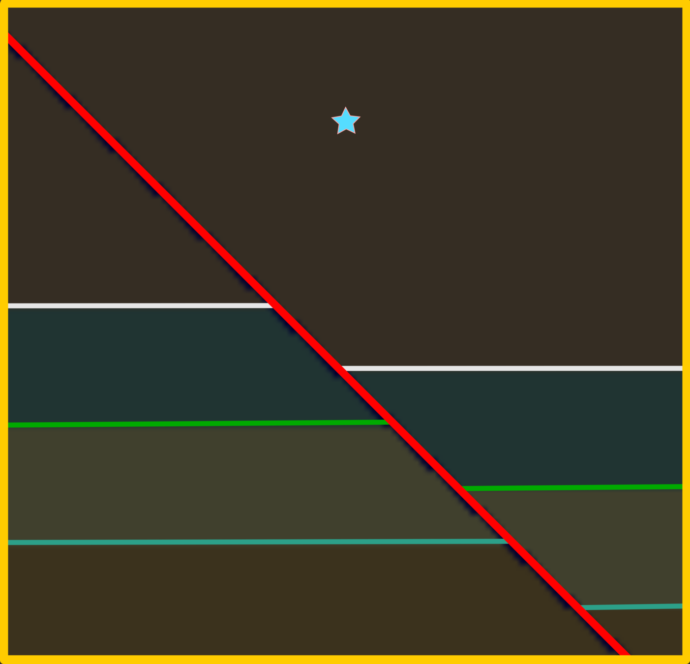
Wave Propagation in Geological Structure
model
time step
17
time step
21
time step
27
time step
37
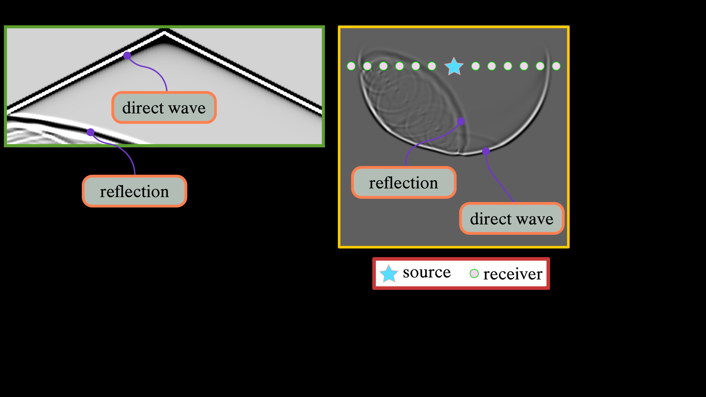
Once the direct wave strikes the zone fault, it will reflect some energy, probably back to the surface, and residual energy will transmit to the adjacent media. Noticeably, on the left part of the footwall, the spherical wavefront begins to distort, whereas, on the hanging wall, it still maintains the feature.
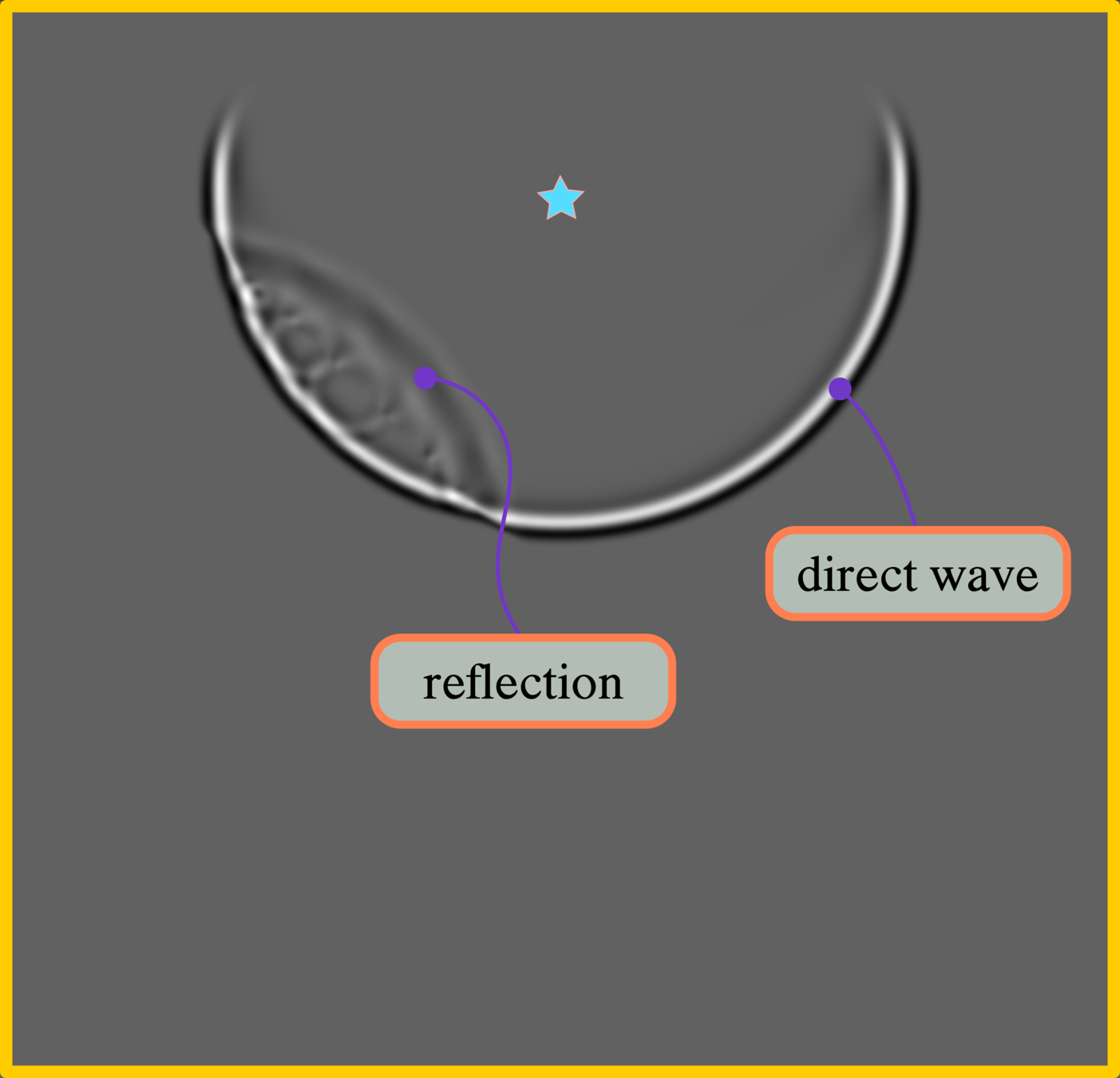
Wave Propagation in Geological Structure

model
time step
17
time step
21
time step
27
time step
37
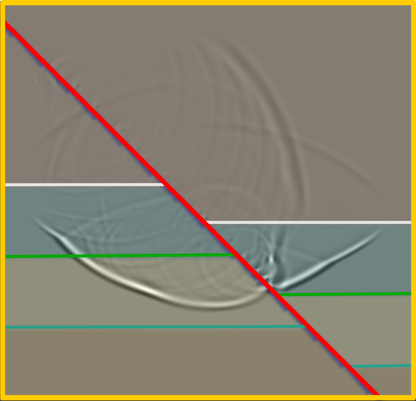
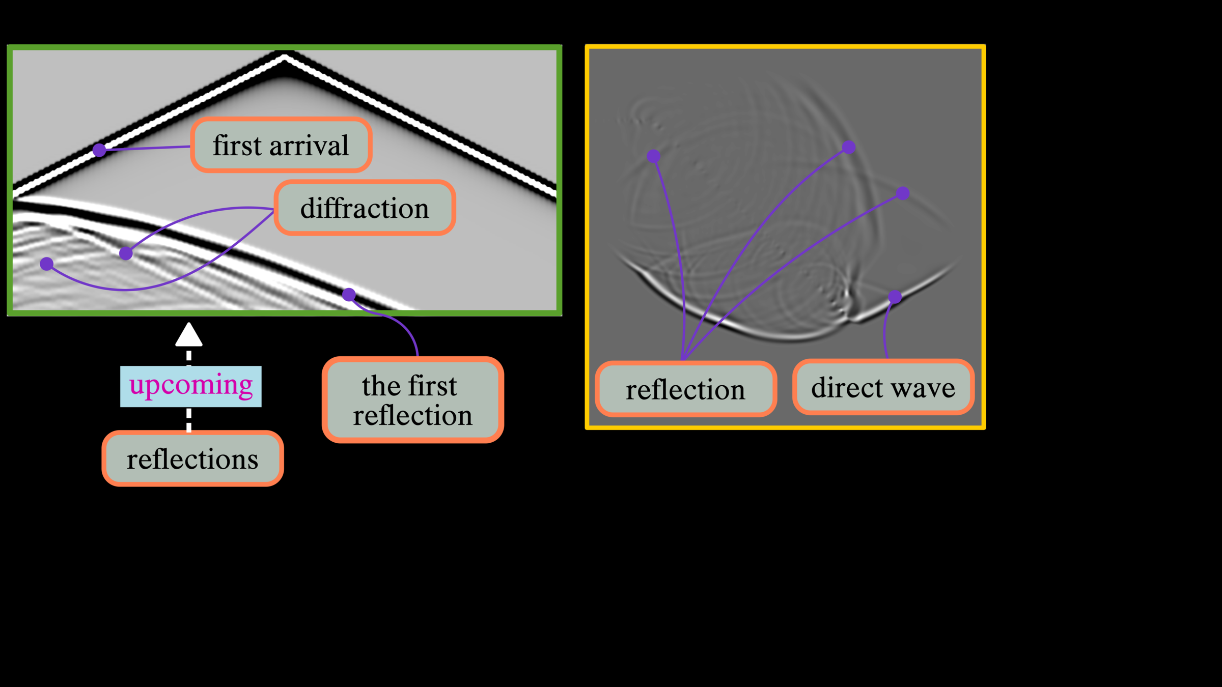
In this time step, the zones containing high impedance contrasts demonstrate reflections such as the fault zone and the first layer (green line). The complex waveform generated from the internal fault body oscillates diffracted waves that are the primary component of the reflection.
Wave Propagation in Geological Structure
model
time step
17
time step
21
time step
27
time step
37
In this snapshot, the reflections from different layers represent strong amplitudes possessed hyperbolic-like features. The diffraction reveals in several places, and these waveforms might be stacked during the migration process as signal or noise, which depends on the multifactor.
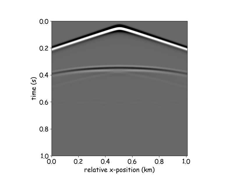
Receiver
time step
17
time step
27
time step
37
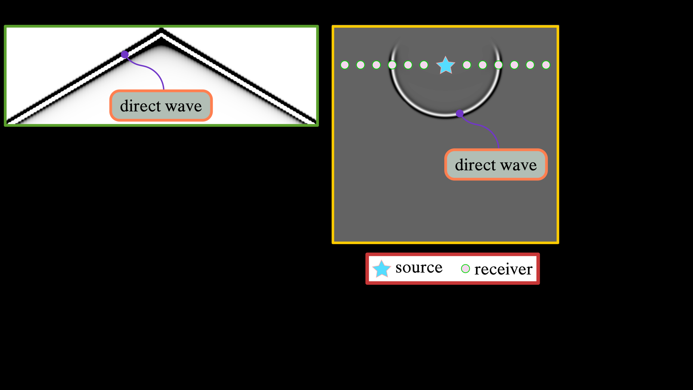
The direct wave, or the first arrival, is the wave that first arrives at a receiver and generally shows the strongest amplitude. This waveform is removed during the preprocessing in seismic exploration because it provides less subsurface information. Geologists prefer reflected waves that can provide more surface information.
Receiver
time step
17
time step
27
time step
37
The first reflection arrives later after the direct wave mostly passes through receivers. We know that reflection travels in a two-way time, first propagating to a reflector and returning to the receivers on the surface.
Receiver
time step
17
time step
27
time step
37
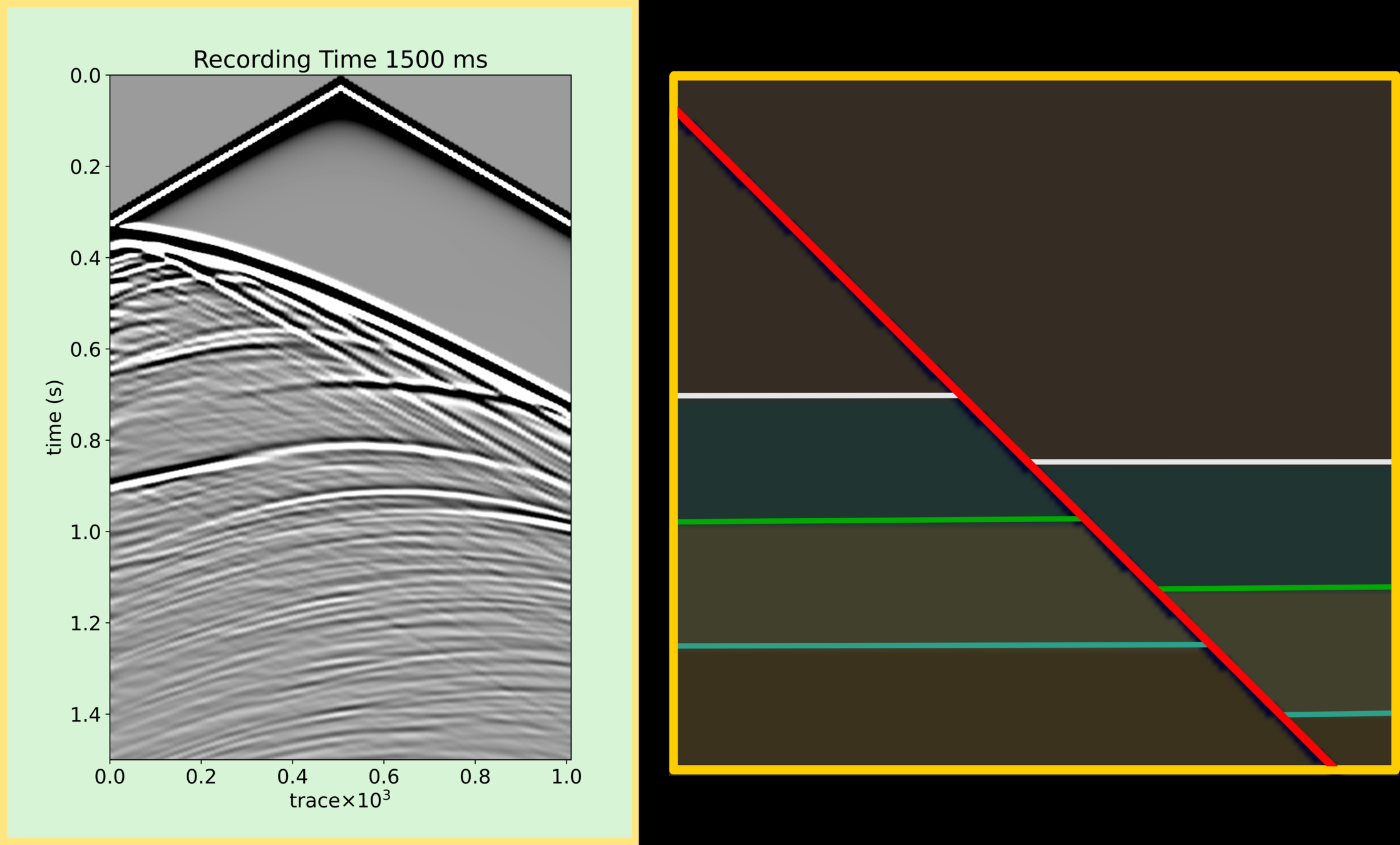
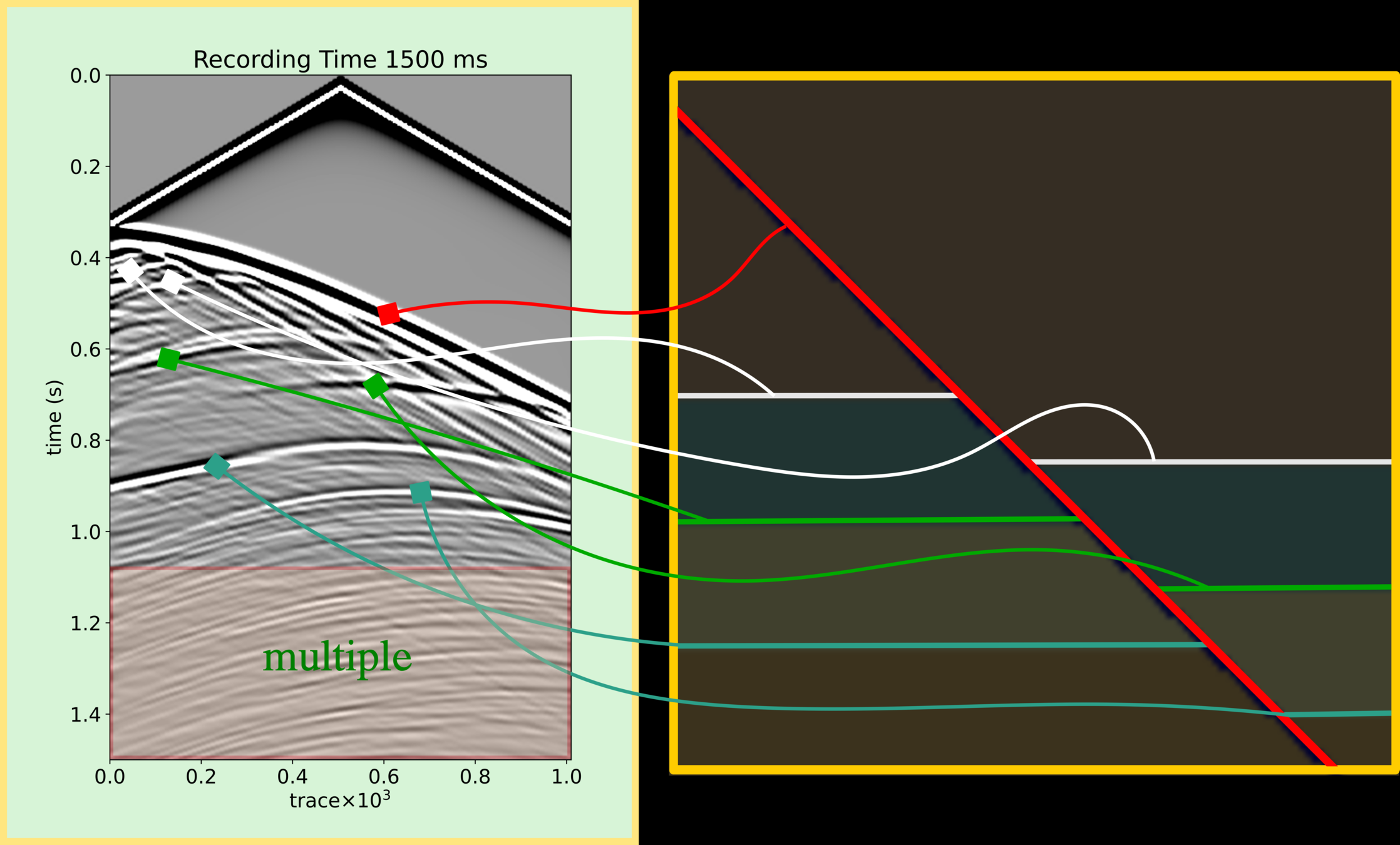
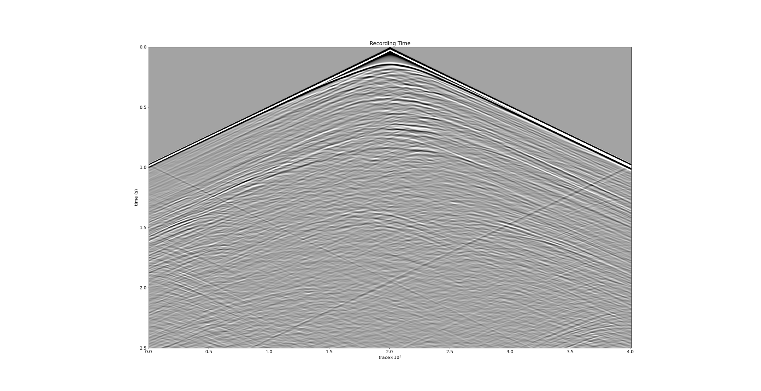
In this recording time, the first reflection reflects at the fault zone, and multiple diffractions are visible underneath this reflection. To correct more subsurface data, we need to increase the recording time, particularly for deep exploration. Commonly, an offshore exploration has a target of approximately five kilometers and a recording time requires up to seven seconds.
Receiver
click
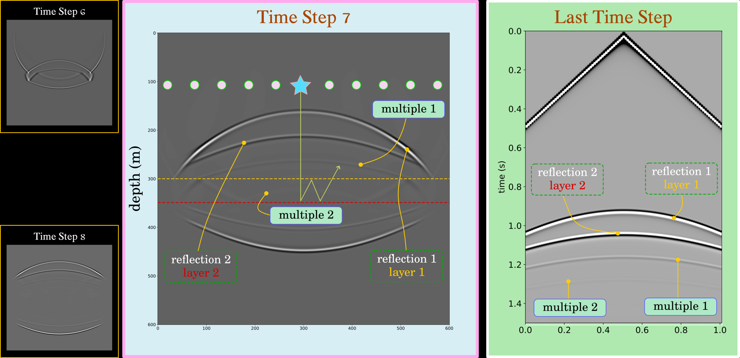
Multiple
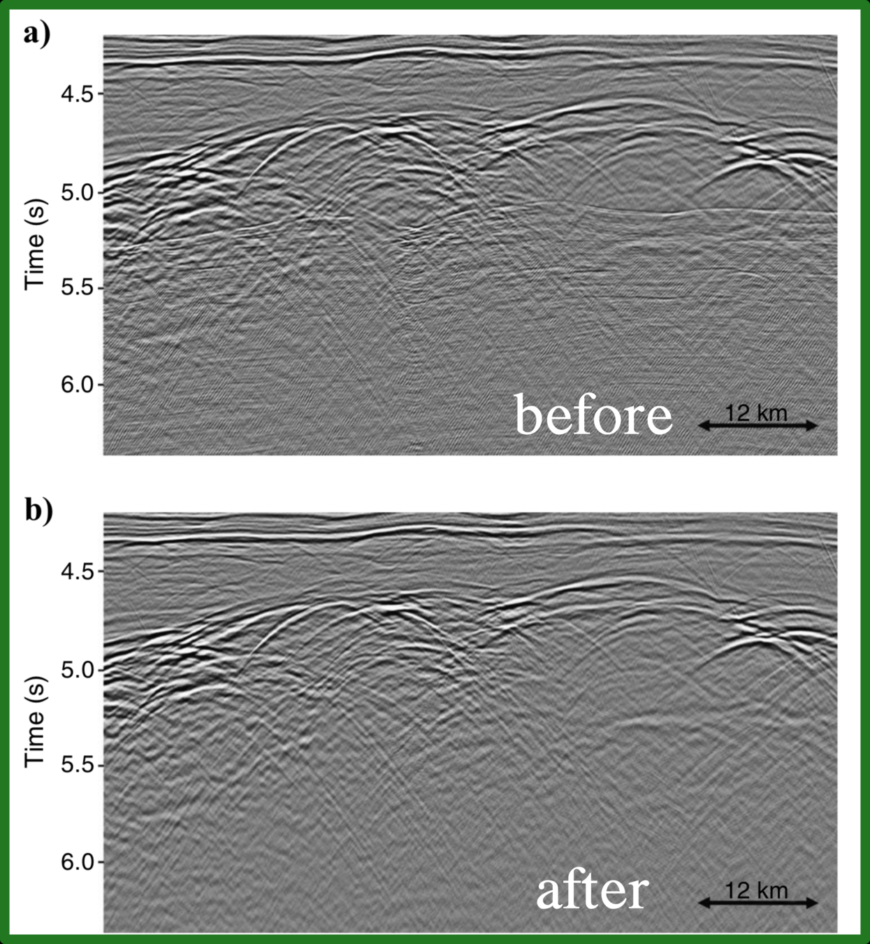
The previous section represents seismic reflection that has downward and upward one time at a reflector. How about there is more than one time of downward or upward during the wave propagation from source to receiver? So this kind of seismic event can refer to multiple. In a seismic image, multiple is considered as noise that is a delusion, causing artifacts in geological horizons (a fake layer duplicated the true event).
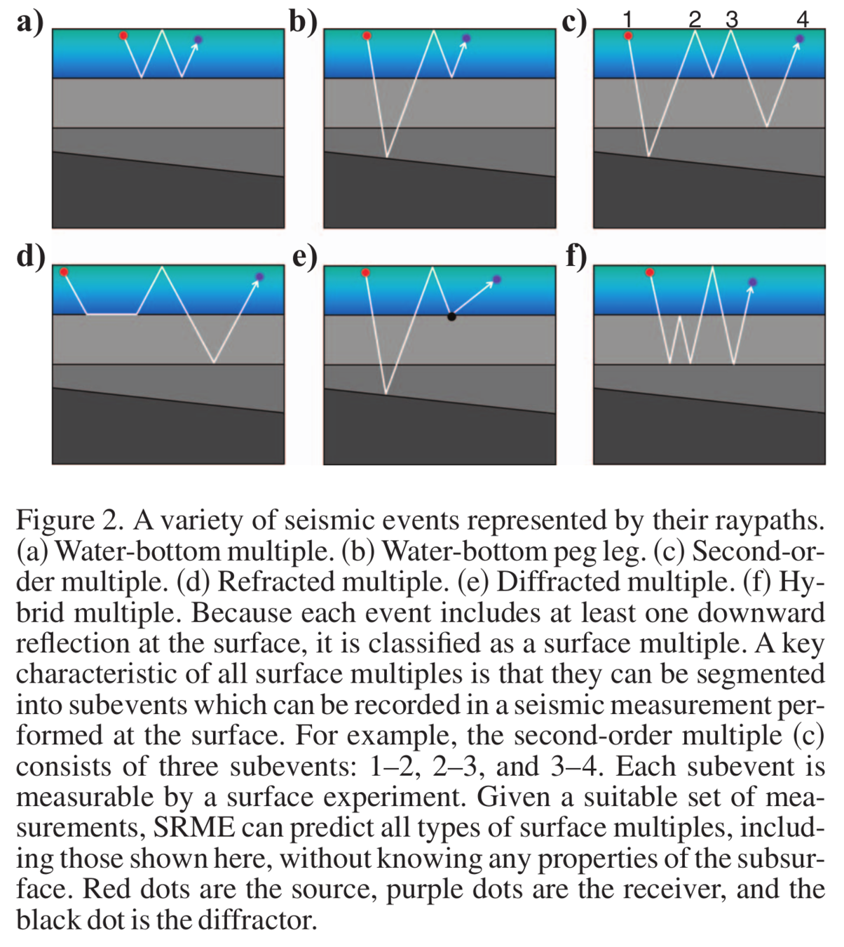
Interbedded Multiple
Multiple in Pre-Stack and Post-Stack Data
click
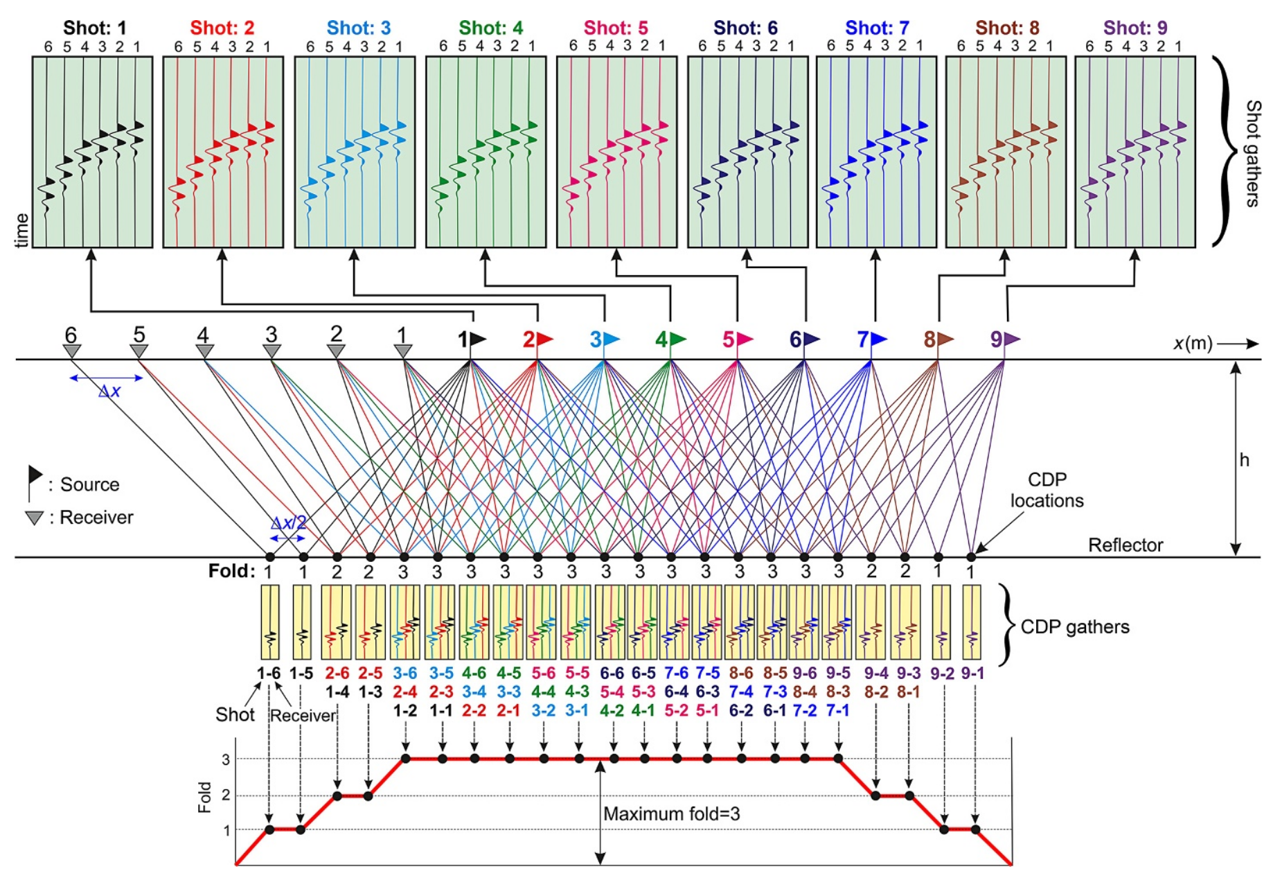
Prestack: Shot Gather
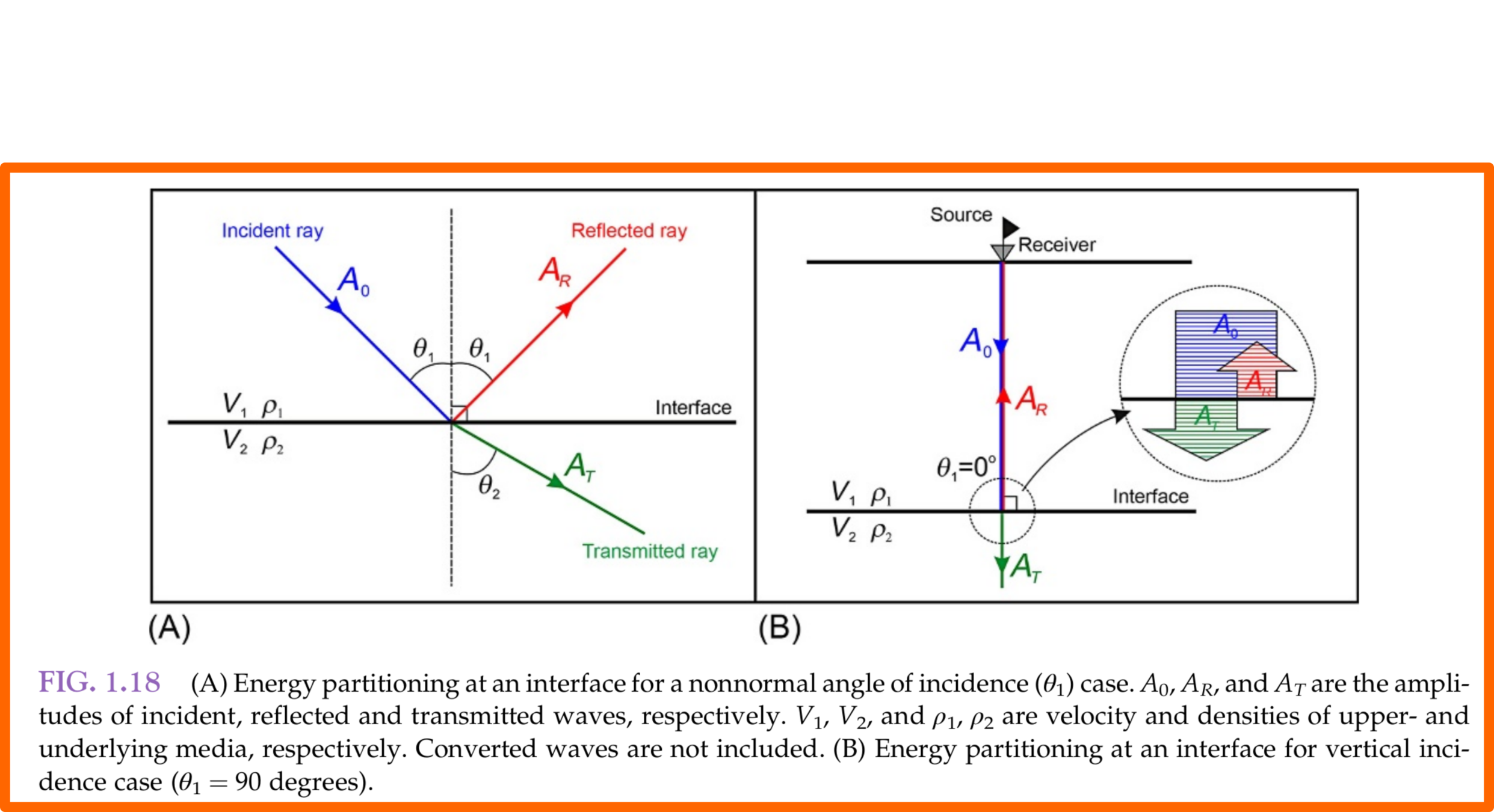
Reflection From an Interface: Acoustic Impedance
Seismic Synthetics
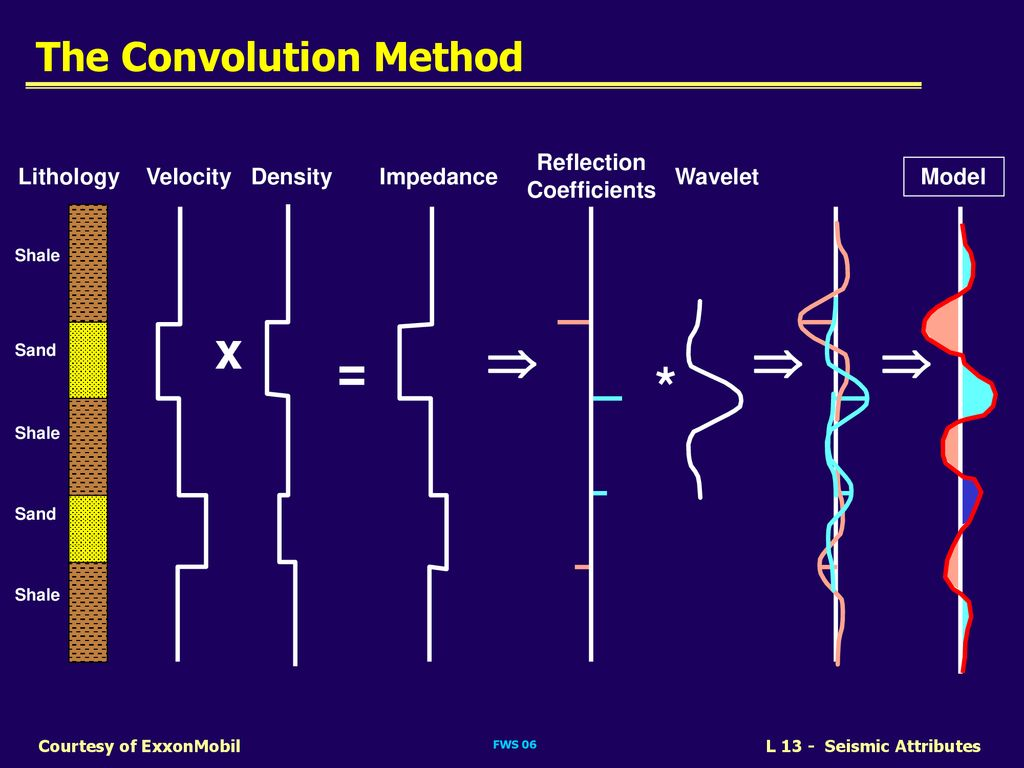


convolution
reflection coefficients
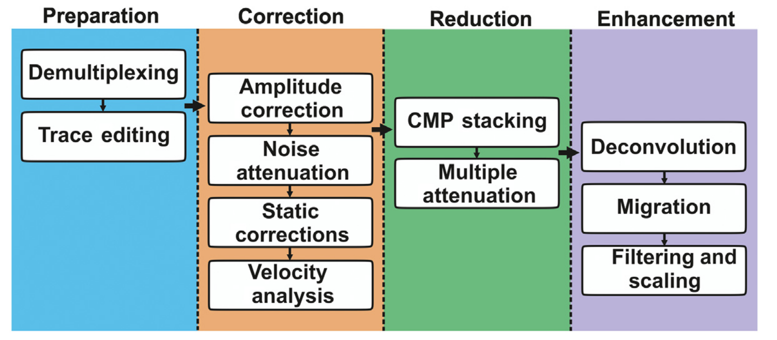
Seismic Imaging Conventional Workflow
Seismic Image From Convolution Method
Seismic Image From Convolution Method
Seismic Image From Convolution Method
Final Exam Guideline
1. Create a seismic-like image using the convolution method. This step can use an outcrop image from the internet or created from the visible geology website.
2. Create one timestep of wave propagation and highlight transmitted waves, reflections, diffraction, and multiple.
3. Create one shot of the geophone and highlight first-arrival and reflection events.
4. Interpret your geological structure based on the synthetic seismic image.
5. Select a few zones and compute dominant frequencies using Fourier transform.
6. What is an acoustic wave, and what does "c" represent?
9. Create a slide that clearly explains of how to create your work.
7. Compute one trace and show reflection coefficient, assuming constant density.
8. Compare low and high frequencies of seismic image. Which image provides better geological structure sense based on seismic image.
CH 5: Ground Penetrating Radar
01_introduction_to_geophysics_22
By pongthep


