2307589
DEEP LEARNING FOR GEOSCIENCE
VERSION 2024.01OVERVIEW


Textbooks

Project Themes

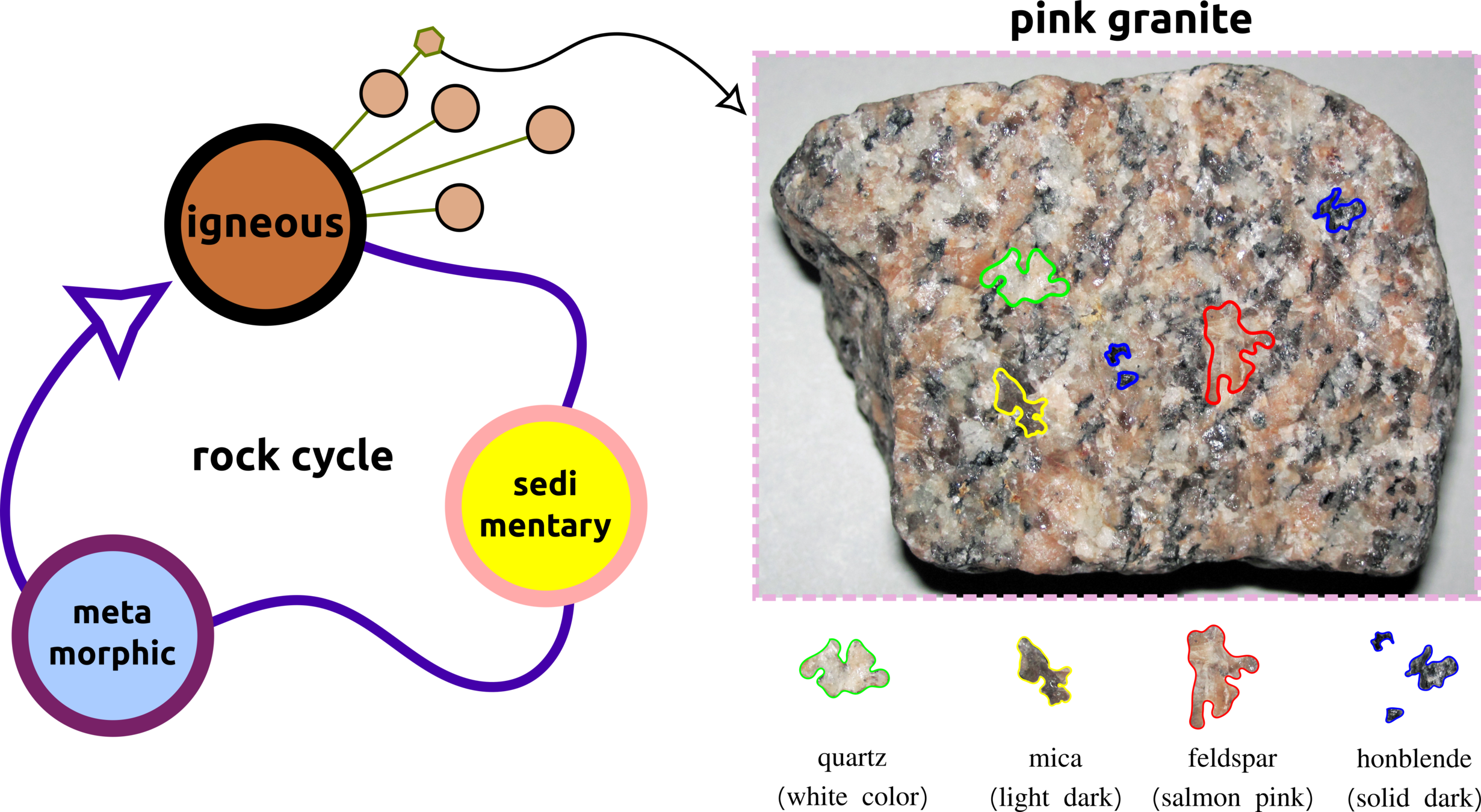
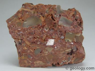
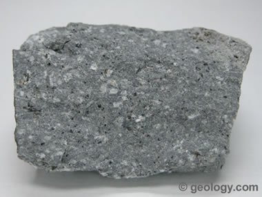
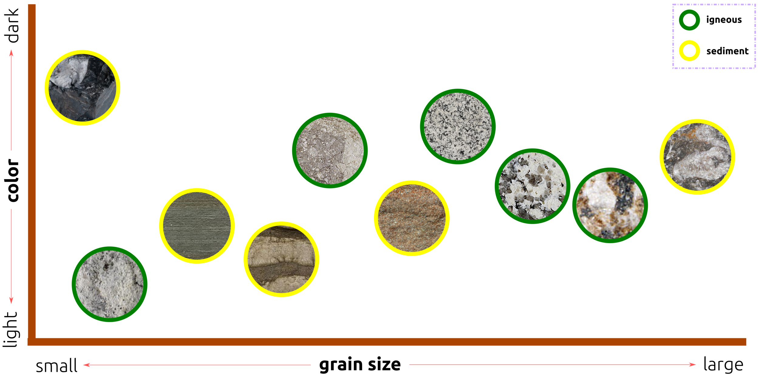
rock classification
INTRODUCTION
Data-Driven Approach
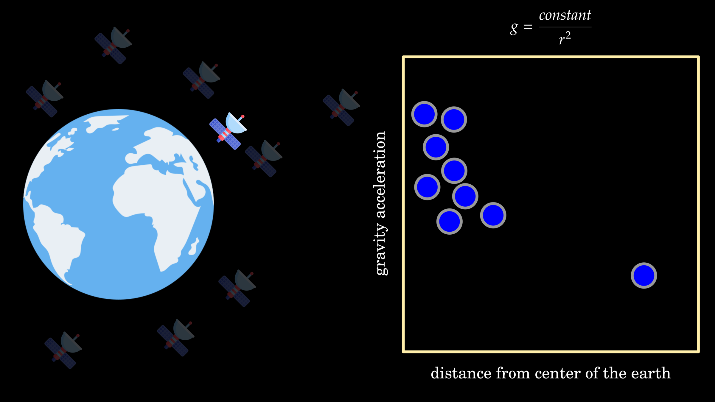
Classic Equation

F = M \times (A + (\alpha_1 + \beta_1))
Modern Equation
theory-driven approach
data-driven approach
ML and DL algorithms
fitting data into equation
deriving equation from data
theory driven
data driven
AI Family
artificial intelligence
data science
deep learning
supervised learning
unsupervised learning
geometric deep learning
machine learning
data analytics
big data
AI Family
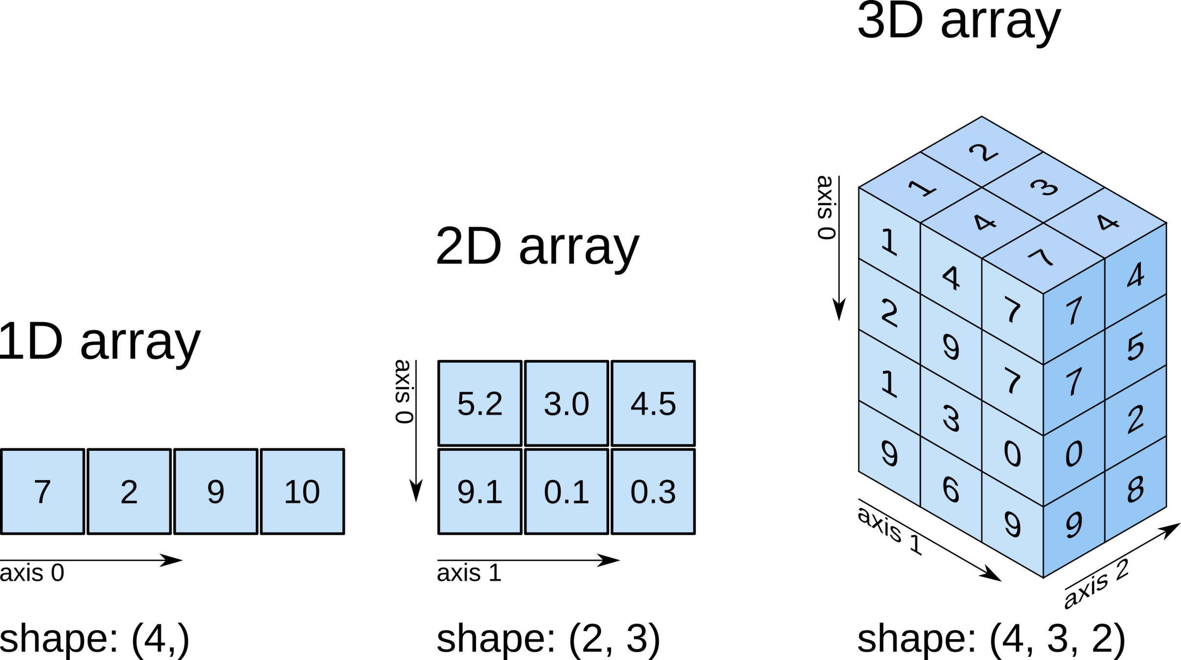
Scalar, Vector, and Matrices
Supervised vs Unsupervised Learning
Supervised vs Unsupervised Learning
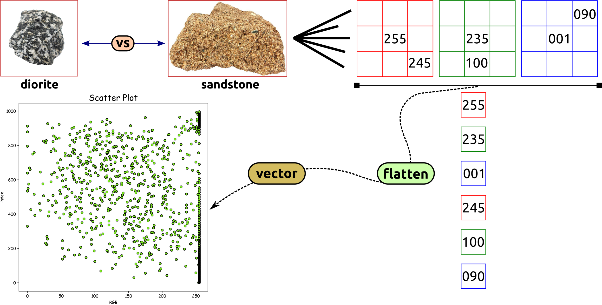
Scattered Plot: Color Intensity and Index
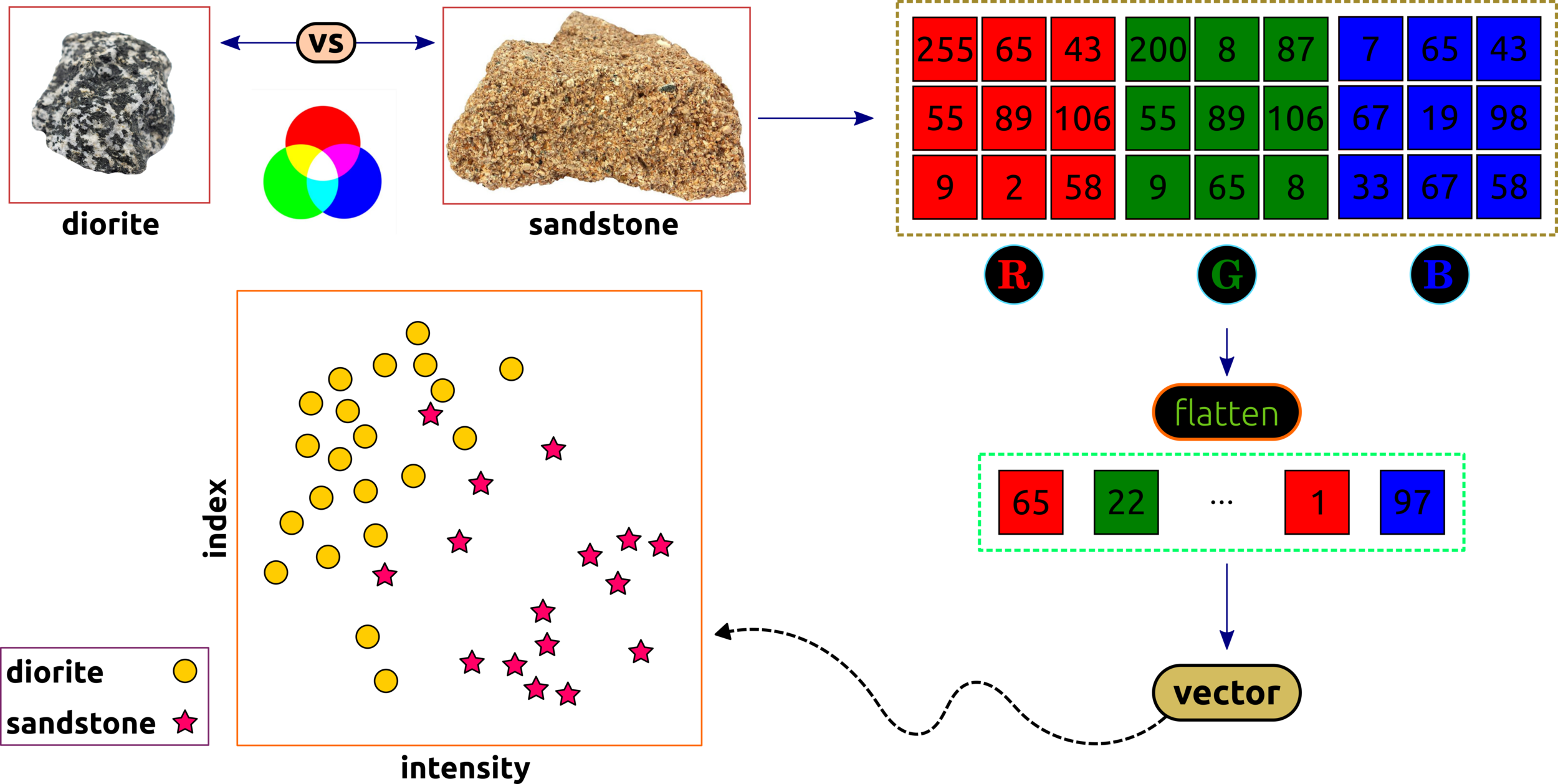
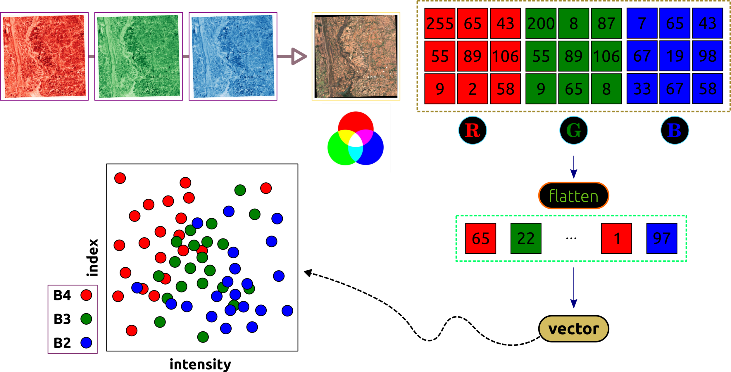
Data Transformation: Image to Scatter Plot
Data Transformation (Satellite Image)
Unsupervised Learning (K-means)
input data
locate centroids
measure distances
relocate centroids
distance equal threshold
end
yes
no


find the shortest paths between each data point and centroid.
yes/no condition, the program will end if the shortest distances between centroids and data points equal the threshold (near 0)

done! good job
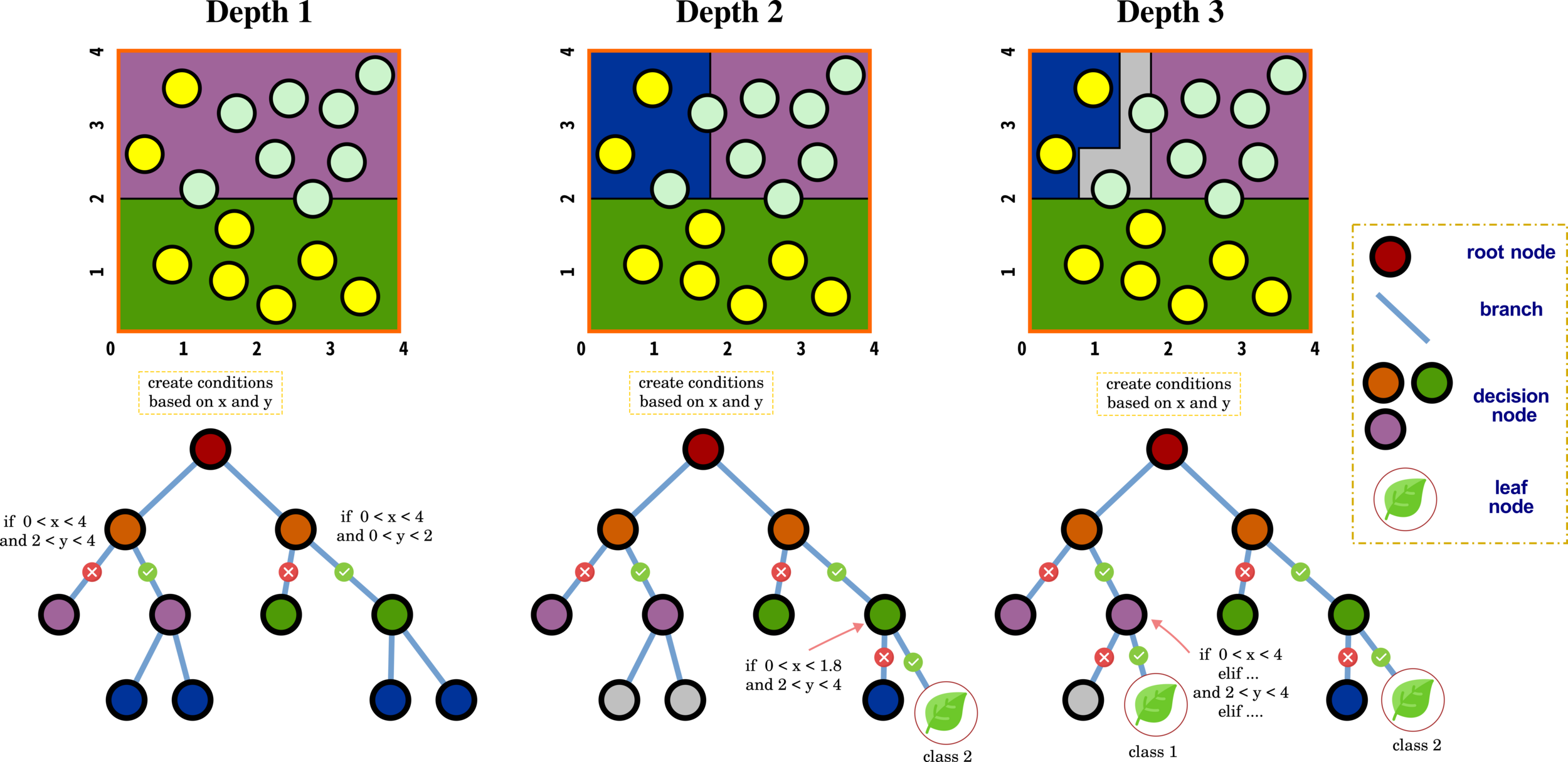
Decision Tree
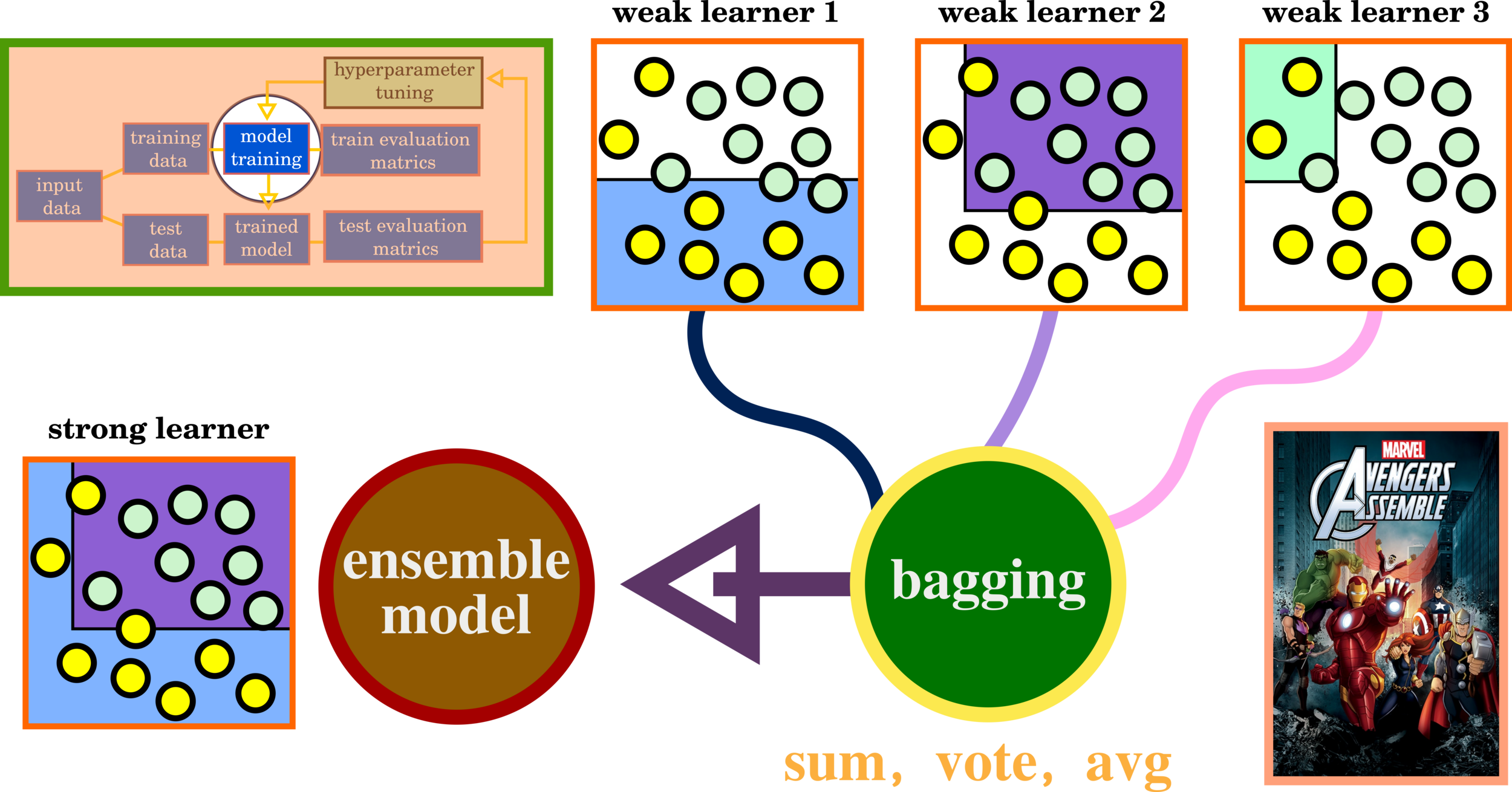
Ensemble Learning: Bagging
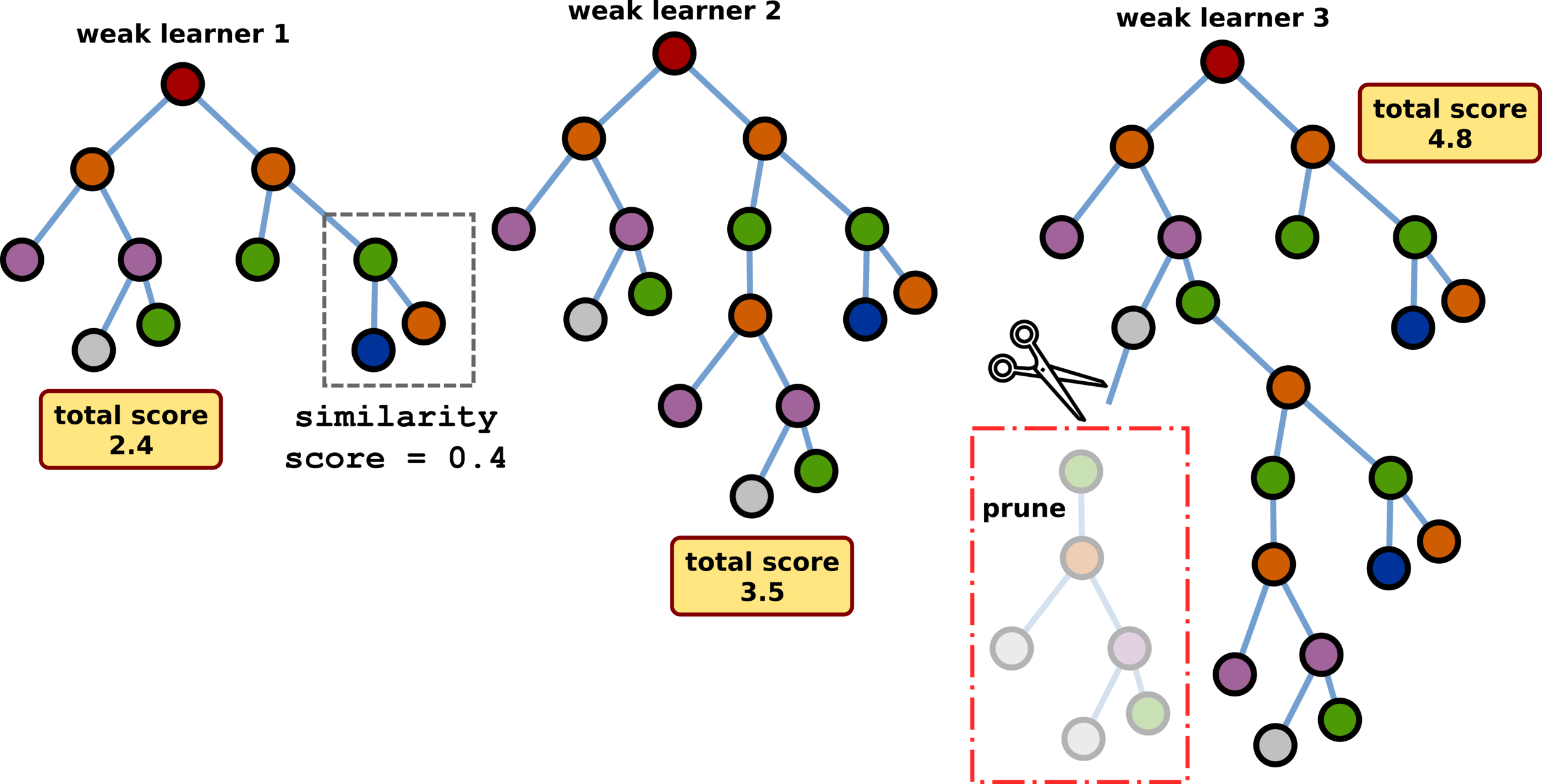
Ensemble Learning: Gradient Boosting
DEEP LEARNING FOUNDATION
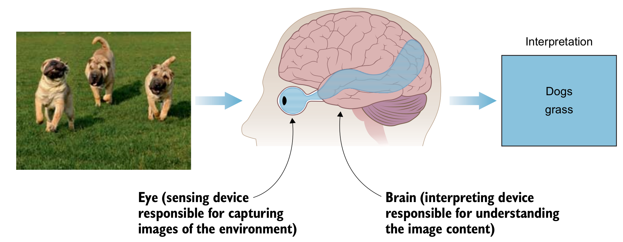
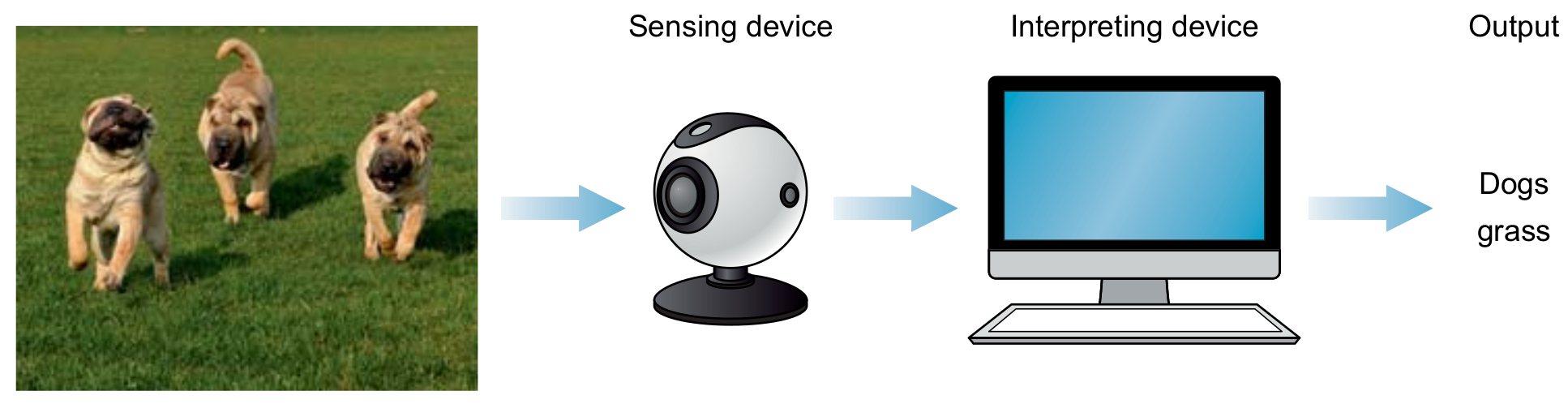
Human and Computer Visions

Biological and Artificial Neurons
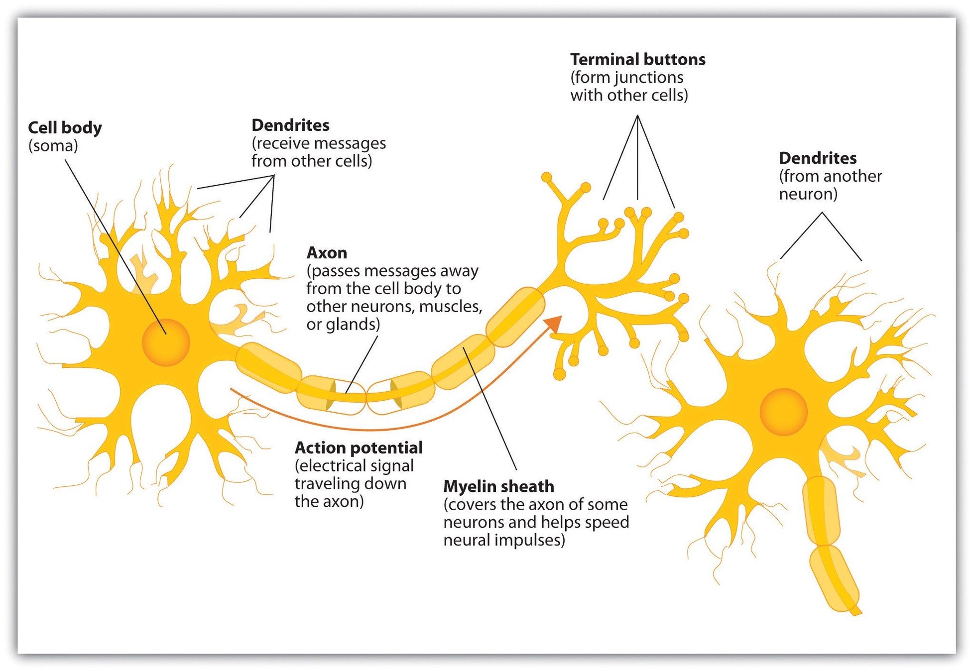
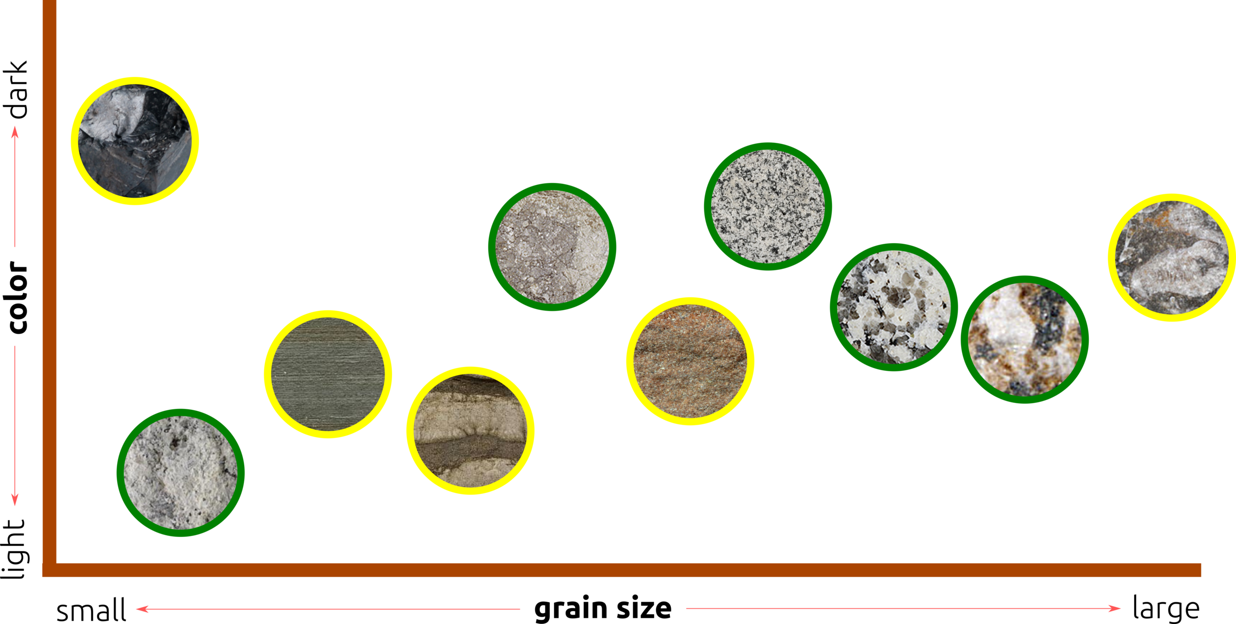
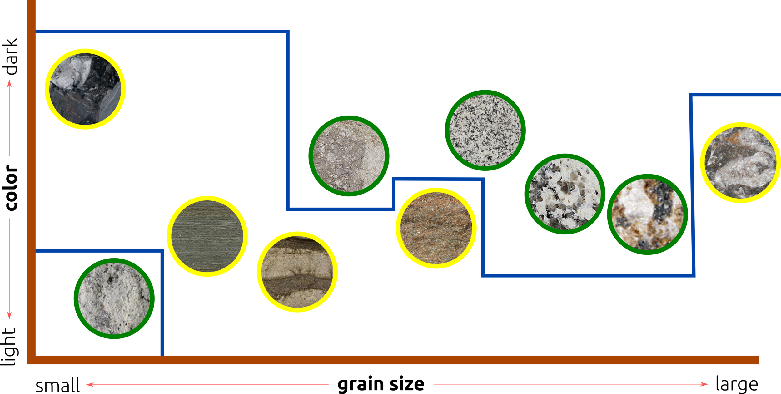
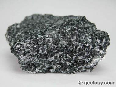
How Do Humans Classify Rock Types?
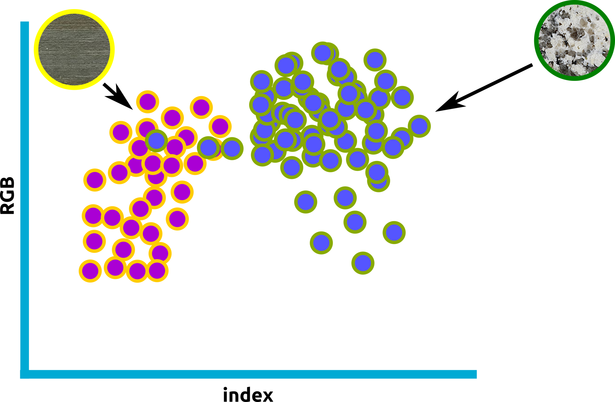
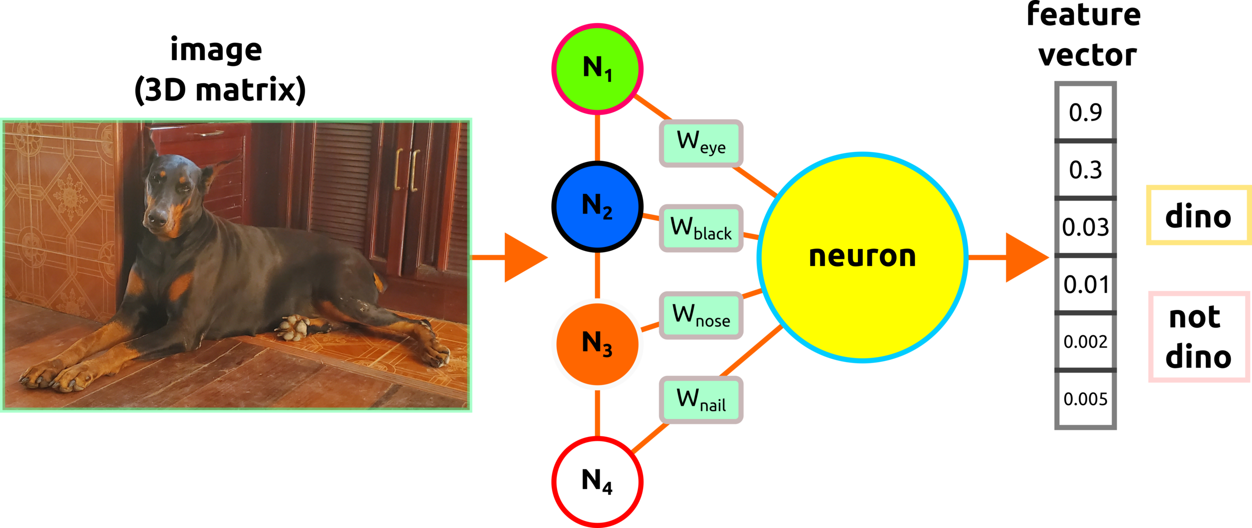
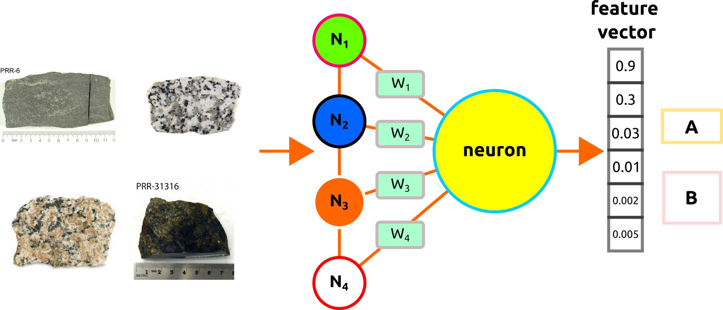
How does a Machine Classifies Rock Types?
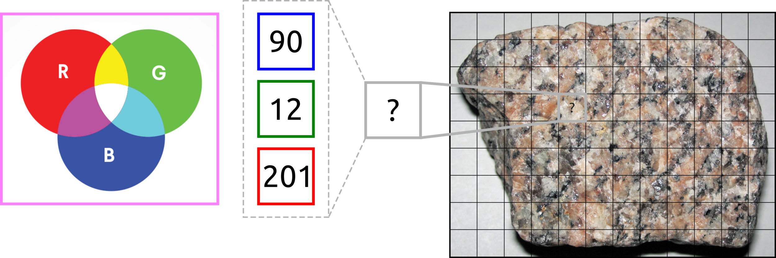
RGB format is used for display on digital screens such as computers, TV, and mobile phones.
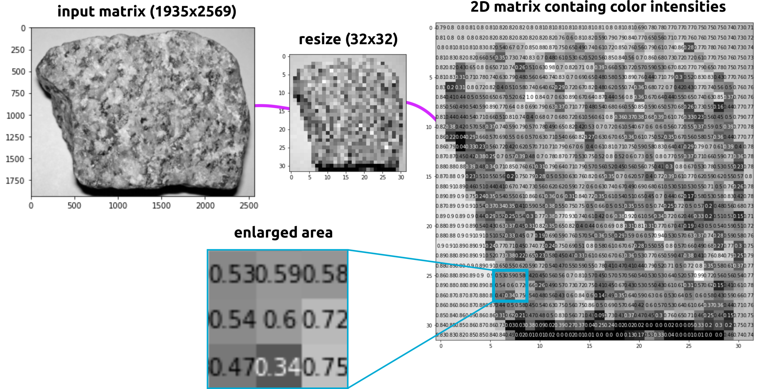
The image and data in computer are functions.
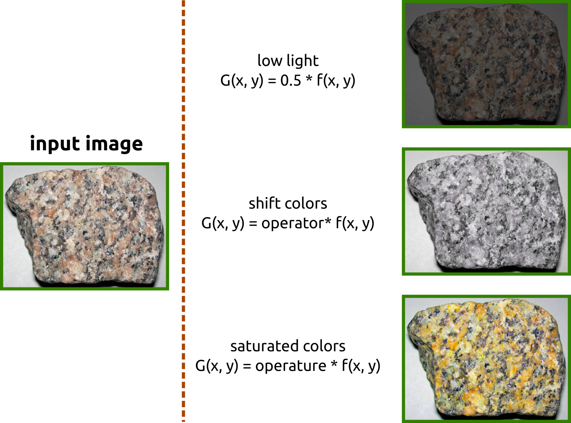
Images are Functions, and Functions are Set of Numbers
Images Transformation
Computer Vision, ML, and DL
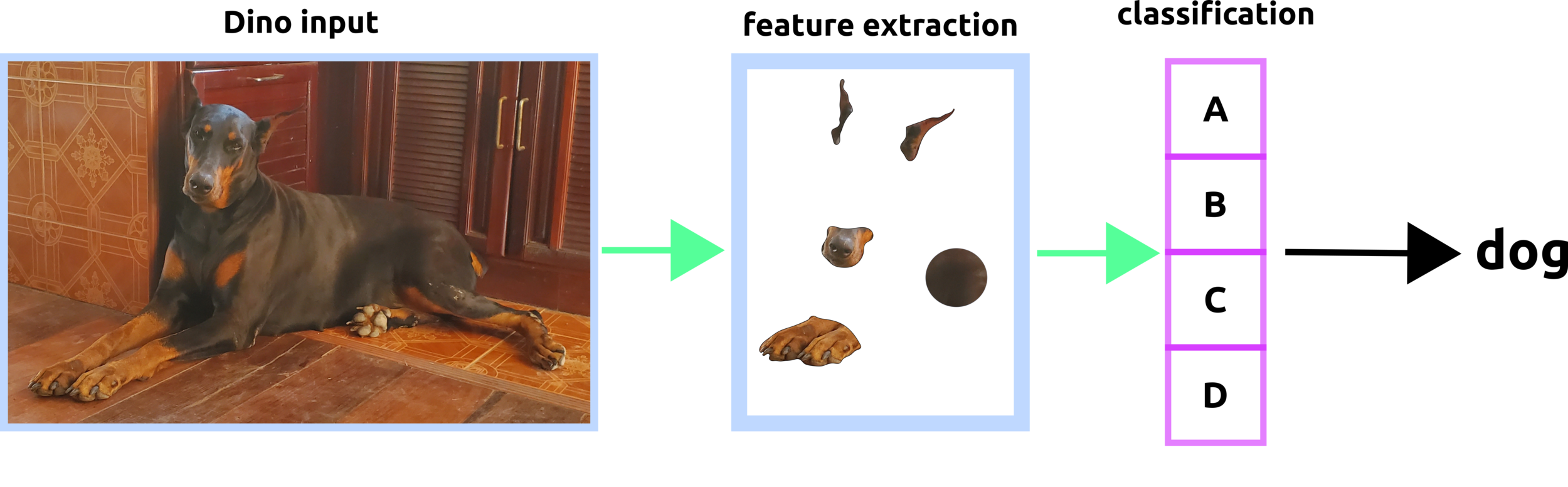
The three methods use different algorithms to extract essential features.
-
computer vision: linear, curve, circle, and colors
-
ML: clustering data
-
DL: neural networks
Some Thoughts: What Are Features Importance?

Perceptron
Deep learning contains several layers, and a single layer is a perceptron.
Some Thoughts: how to weigh this dataset?
MATHEMATICAL BACKGROUND FOR DEEP LEARNING
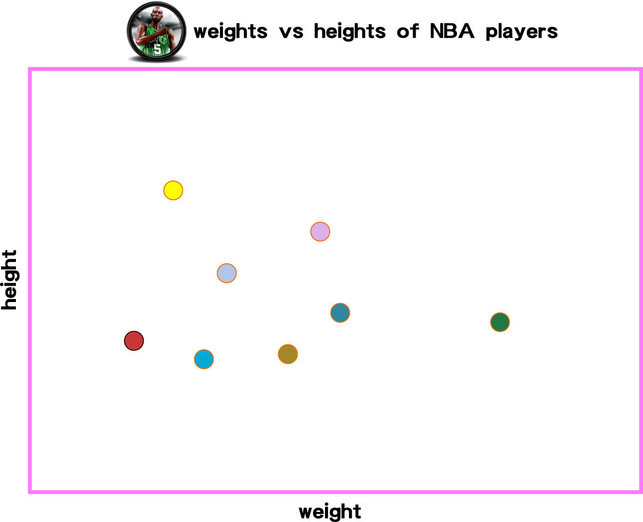
Big Picture: Linear Regression
input
data
iteration
2
iteration
1
iteration
k

The idea of the linear function is to create a function that can predict forthcoming input data. This slide demonstrates three linear functions for measuring the distance among data points and the linear functions.
Which iterated function has the lowest sum of values?
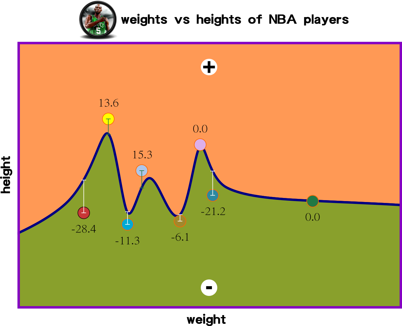
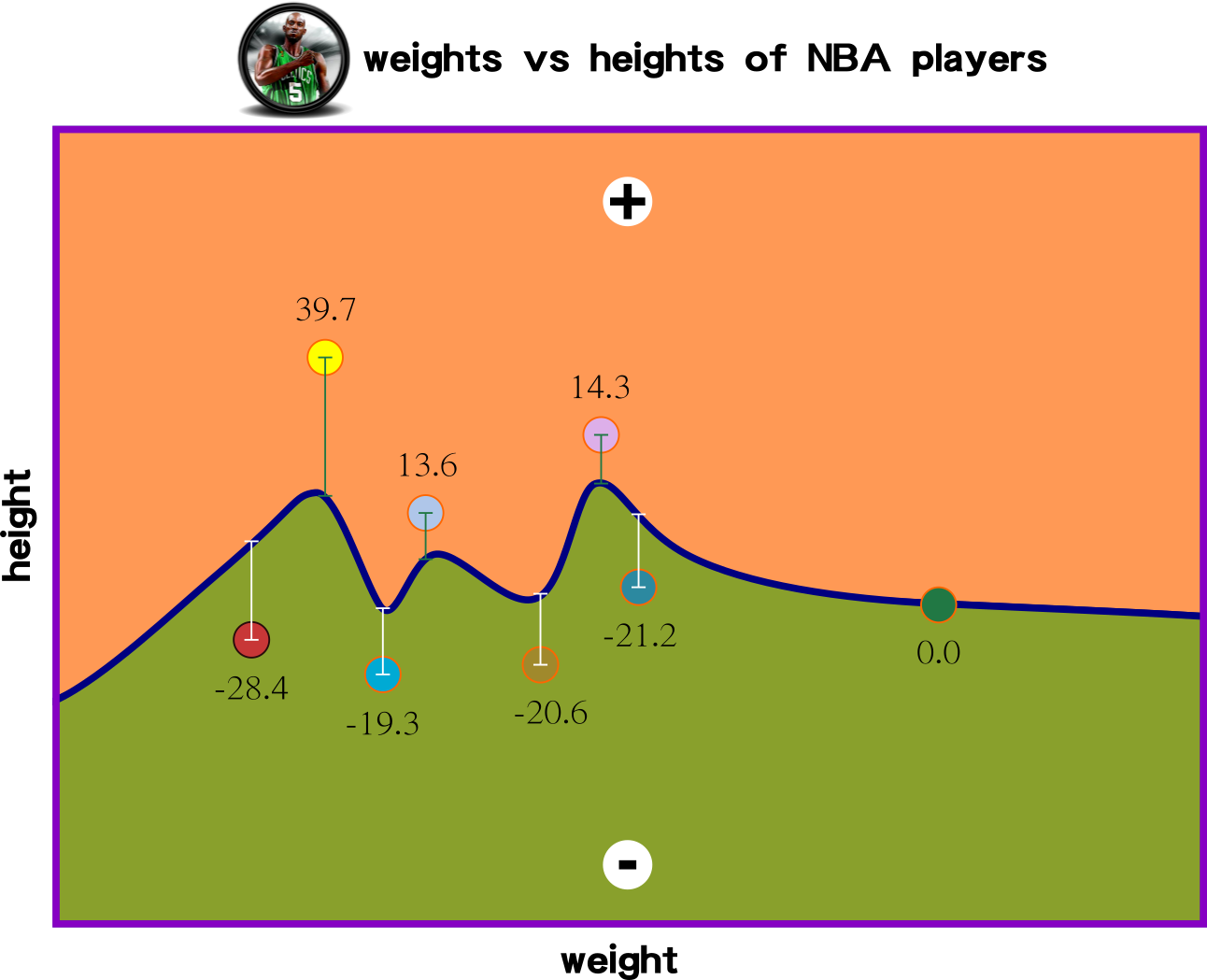
Big Picture: Non-Linear Regression
input
data
iteration
2
iteration
1
iteration
k
the smallest errors are
the best regression
...
how many iteration then that is close to 0?
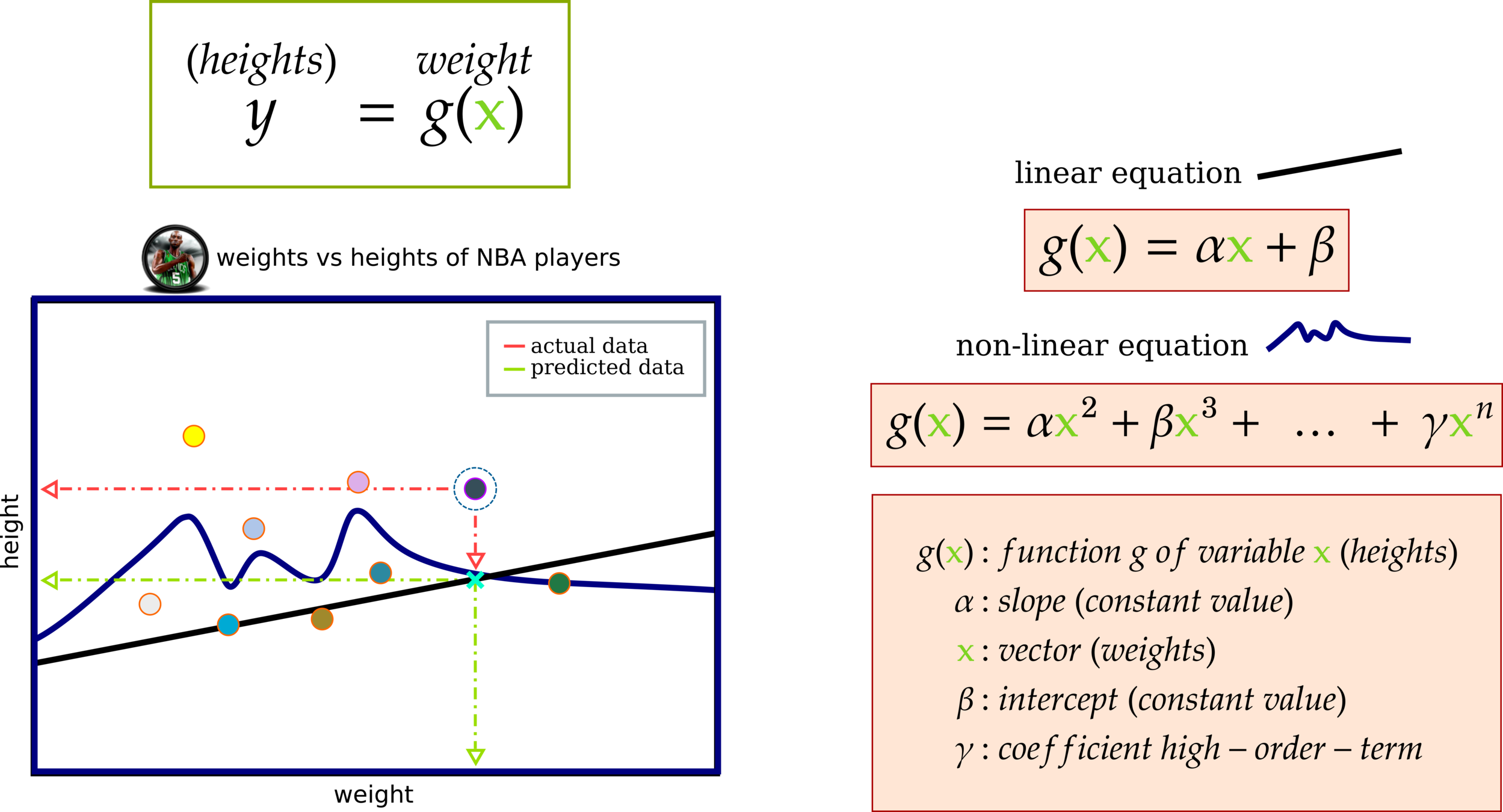
Cost Function: Measuring Model Performance
Function g(x) has a relationship with variable y. This affinity means g(x) might contain several terms to predict the behavior of variable y.
Cost Functions: MAE and MSE
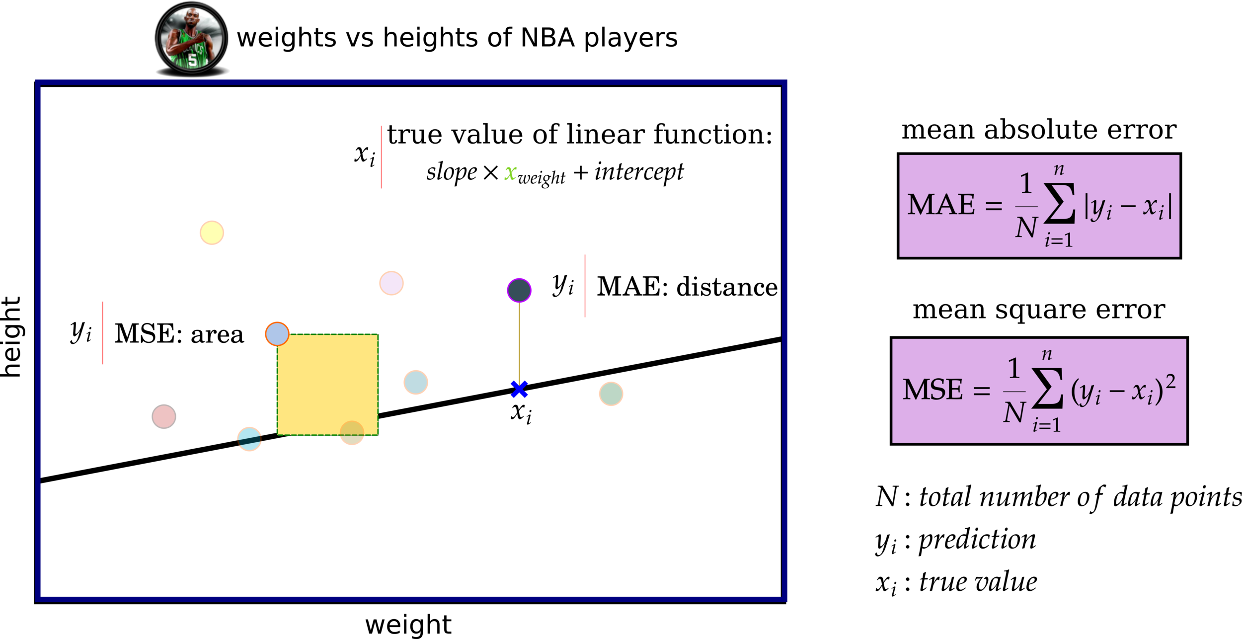
Cost Function Mapping Errors


Rather than trying one pair of slope and intercept, we tested 400 values for each parameter, yielding the result on LHS. On RHS is an example of a selected pair of slope and intercept.
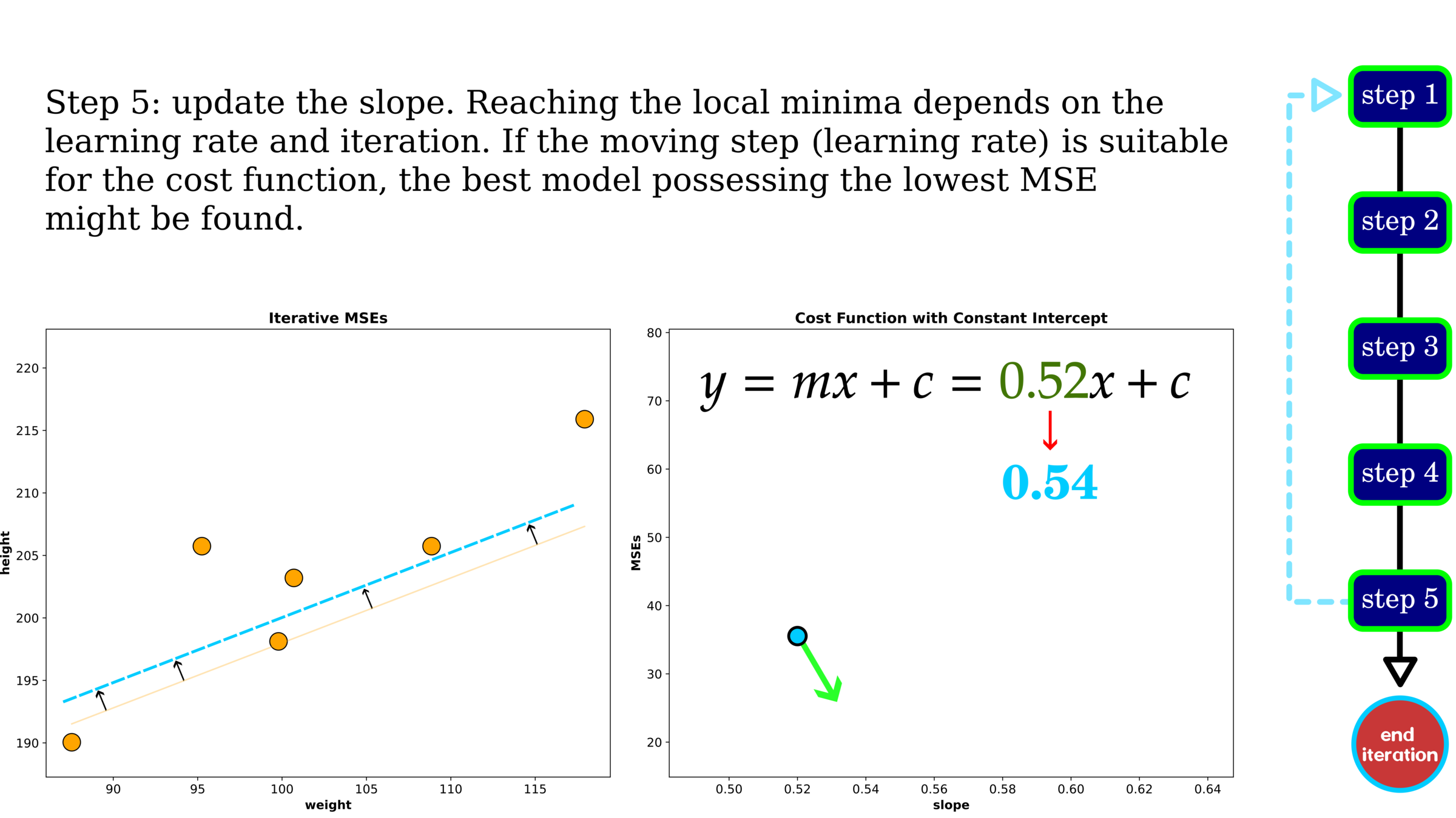
Optimization: Gradient Descent
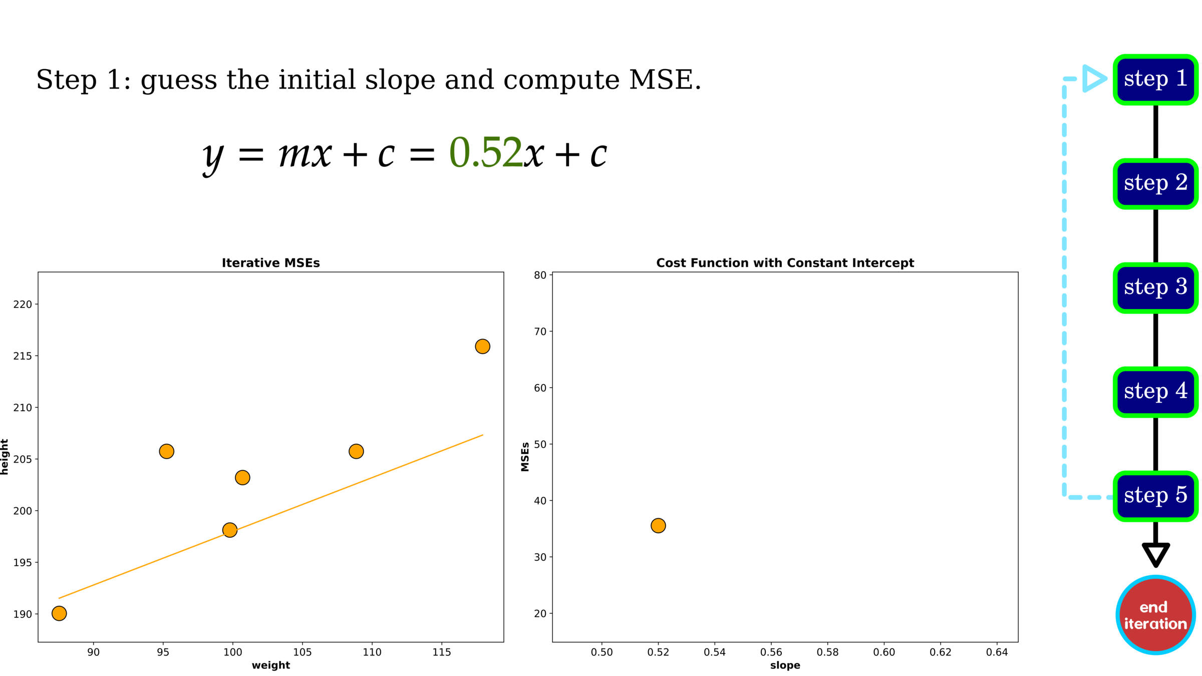
Optimization: Gradient Descent
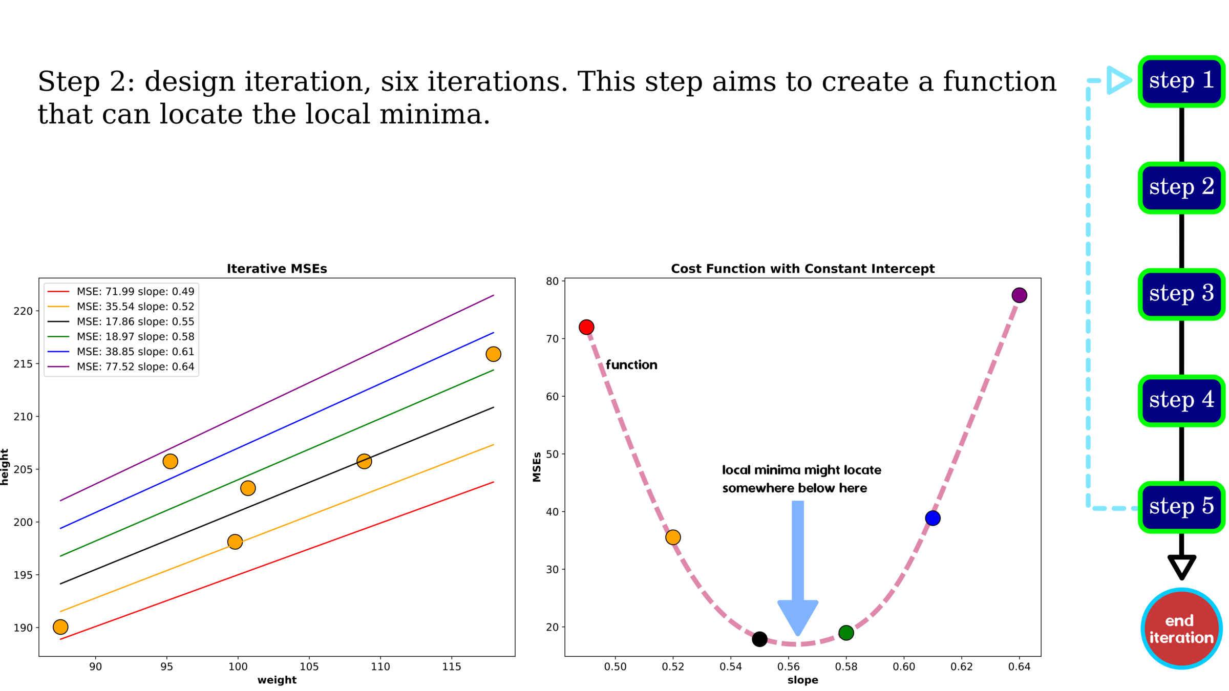
Optimization: Gradient Descent
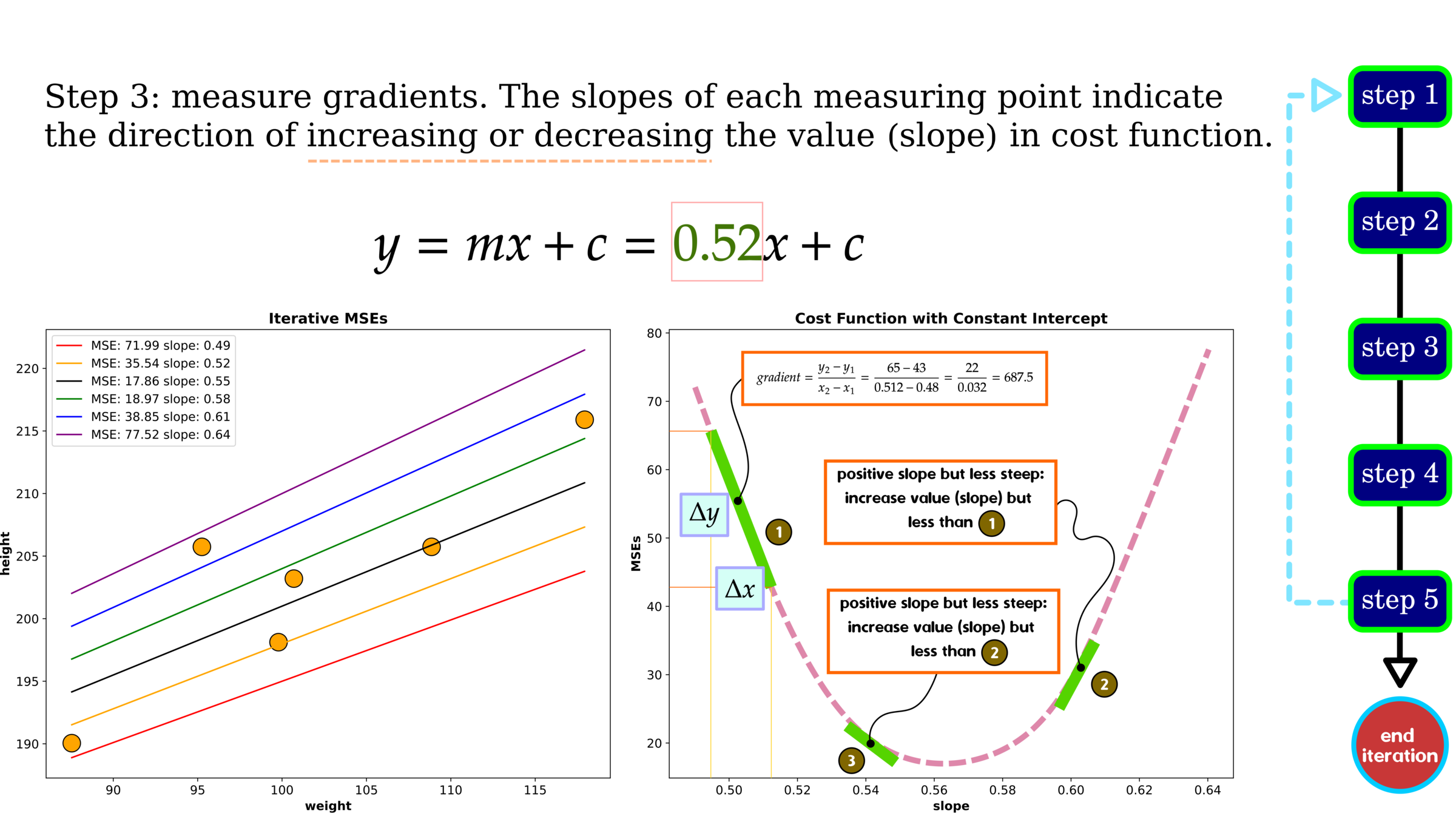
Optimization: Gradient Descent
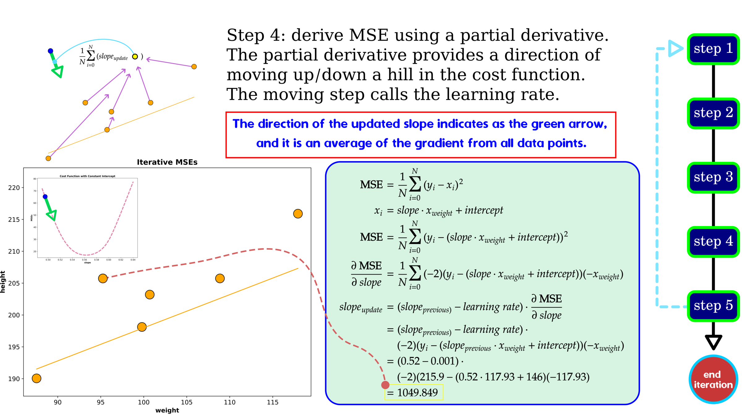
Optimization: Gradient Descent
Linear Regression Using Gradient Descent


Without hyperparameter tuning, gradient descent gives a decent MSE showing higher error than grid search. One data point on cost history indicates trail-out-and-error of tuning variables, slope and intercept. We use the cost history to search the best parameters, and in this example, after iteration 2000, the error is plateauing, indicating that the selected parameter set is found. We should stop searching at this iteration.
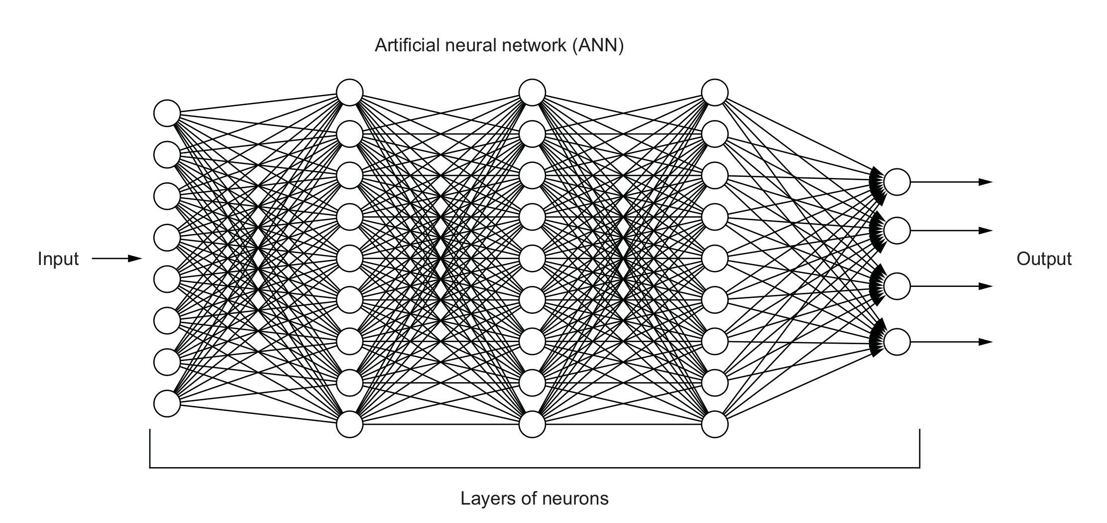
Neural Networks and Deep Learning

FCNN style
LeNet style
Neural networks are the components of DL, which stacks as a multilayer to form a deep learning algorithm.

Perceptron
Perceptron is a part of neural networks and stacking neural networks will form deep learning
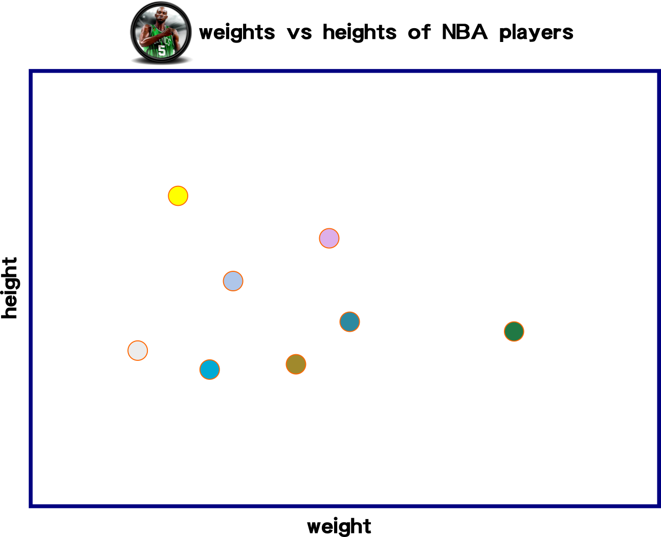
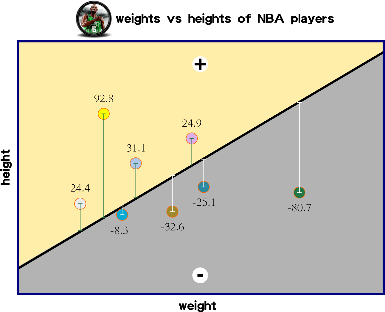
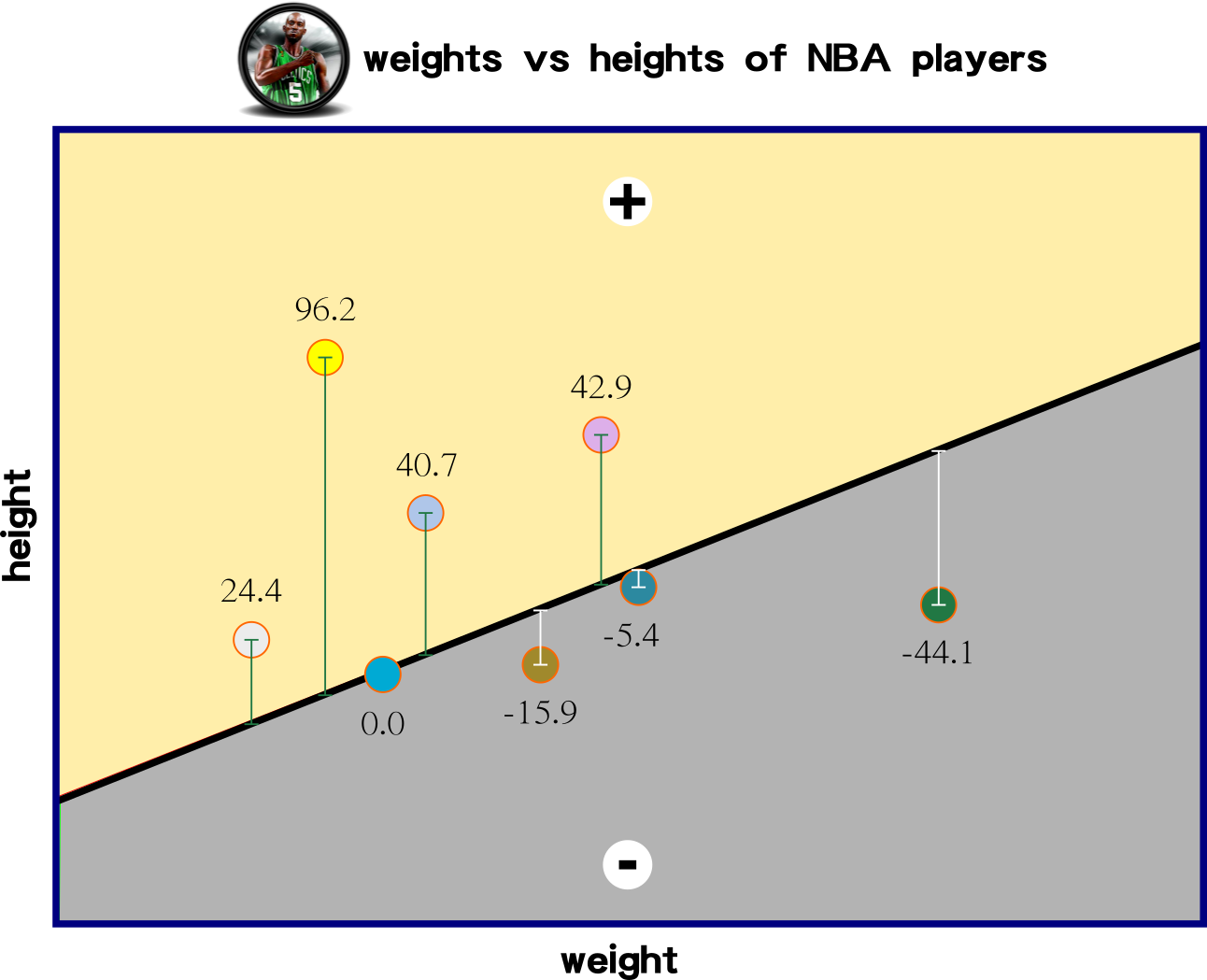
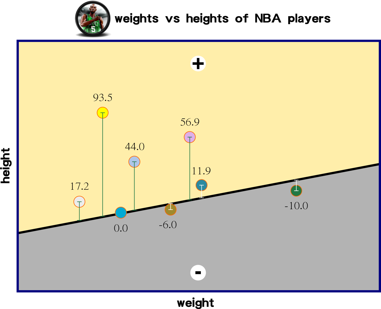
Linear Regression Classification
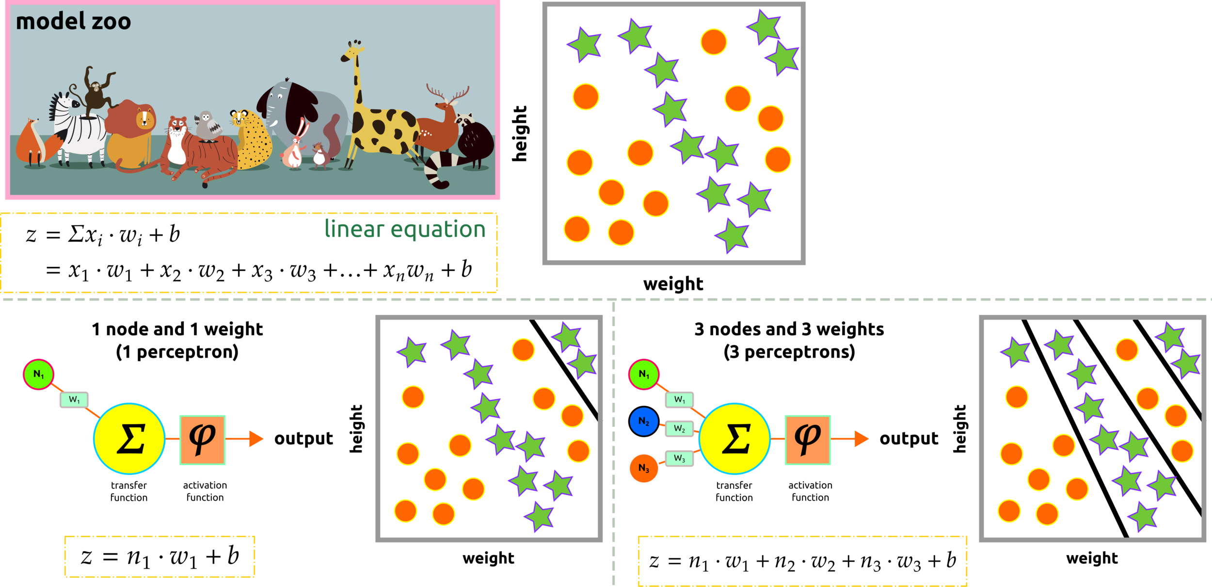
Perceptron uses linear classification to classify a dataset. Model zoo represents animal classification based on two input features, namely height and weight. Clustering the data requires more than one perception; perhaps non-linear classification should implement here.
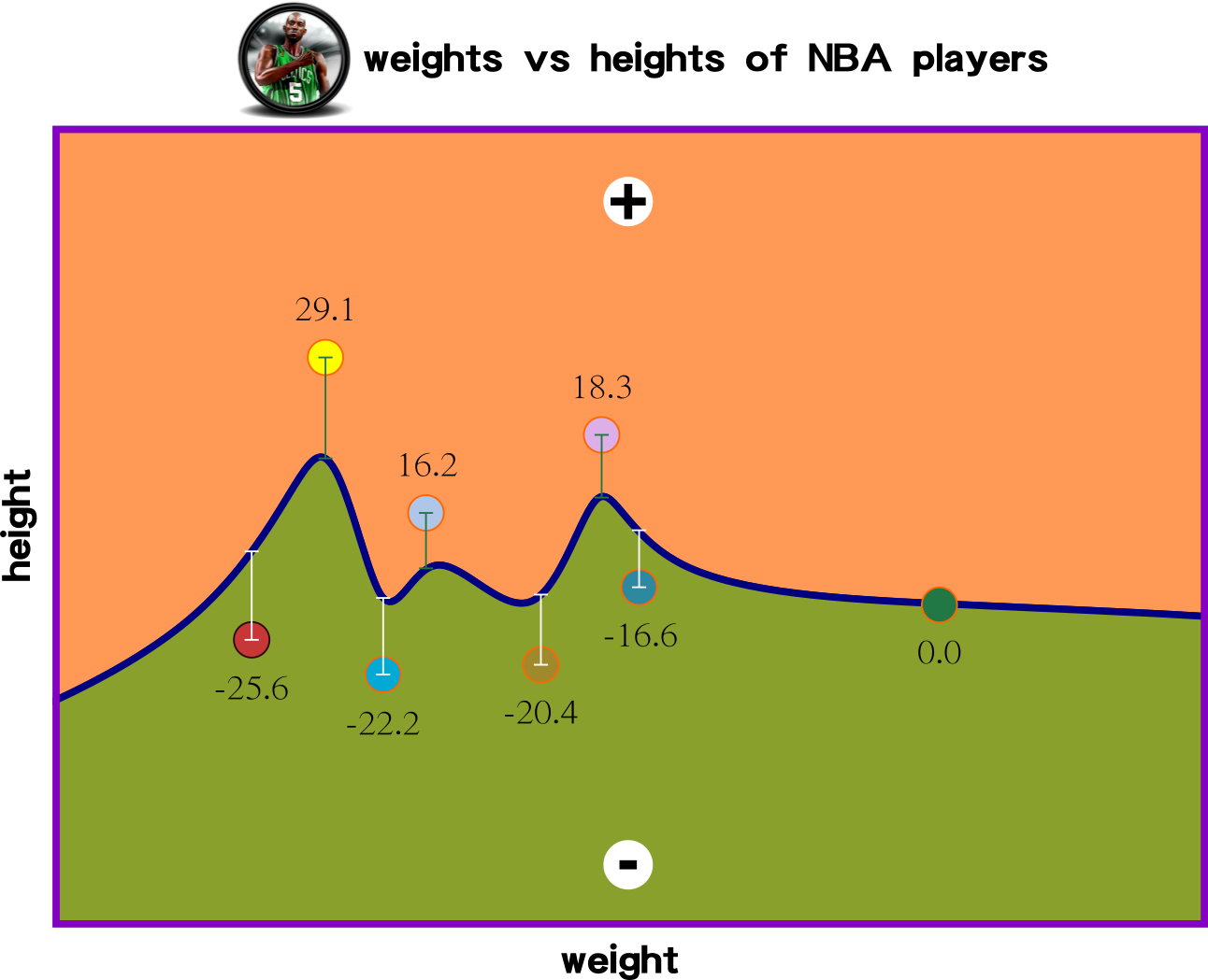
misclassify
(non-linear)
Activation Function: Step Function
misclassify
(non-linear)
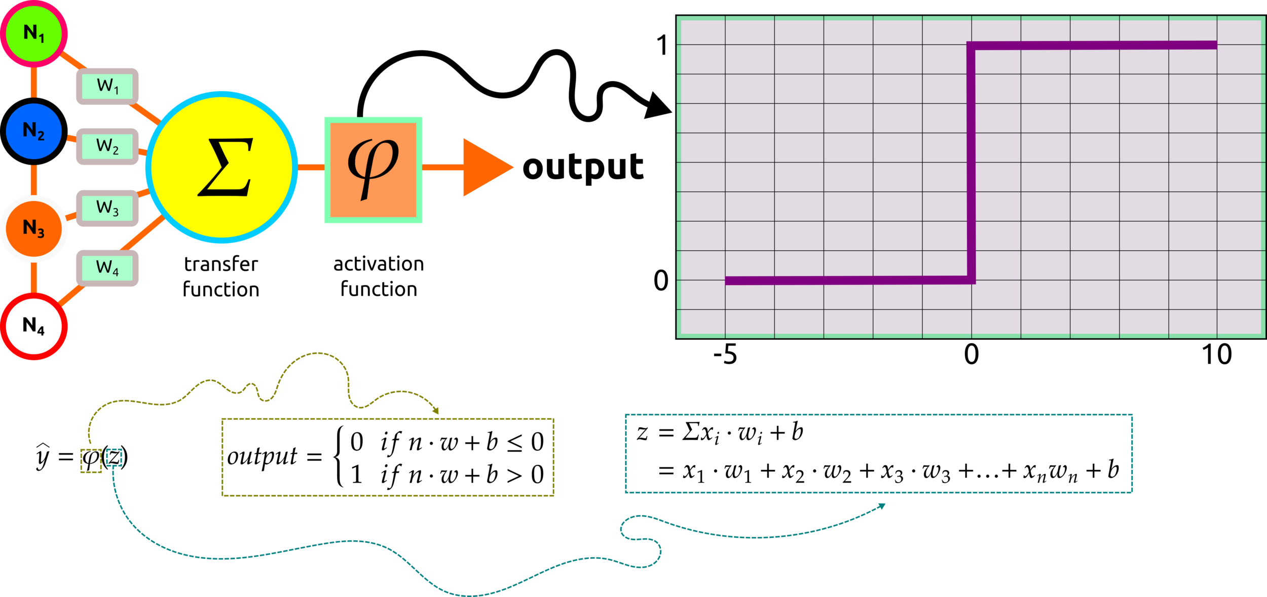
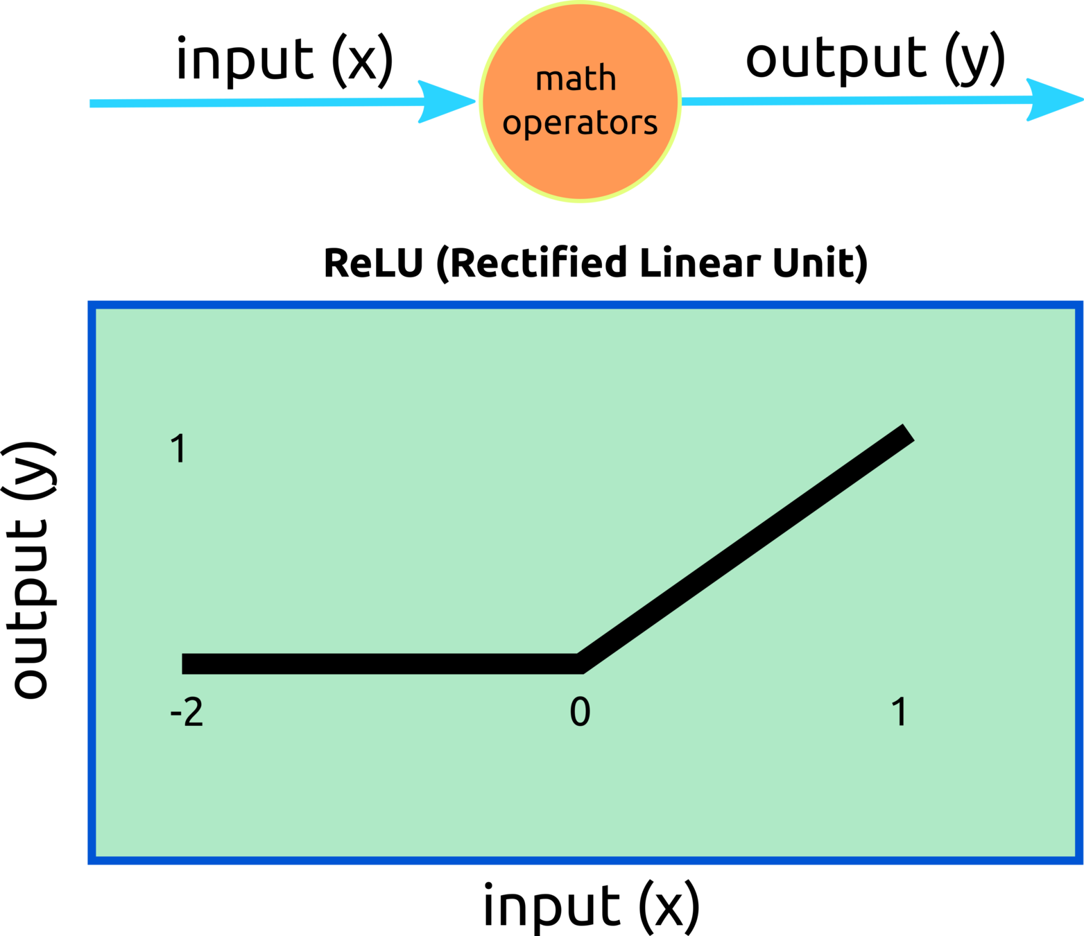
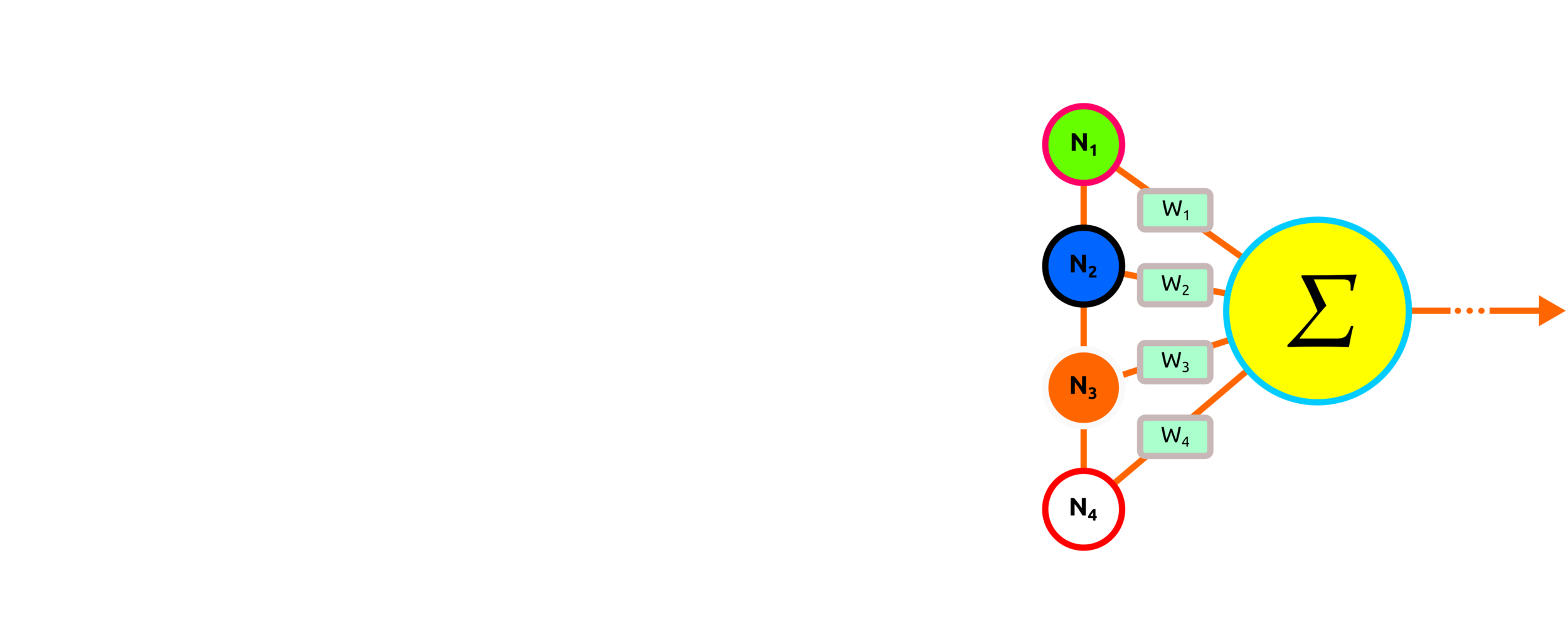
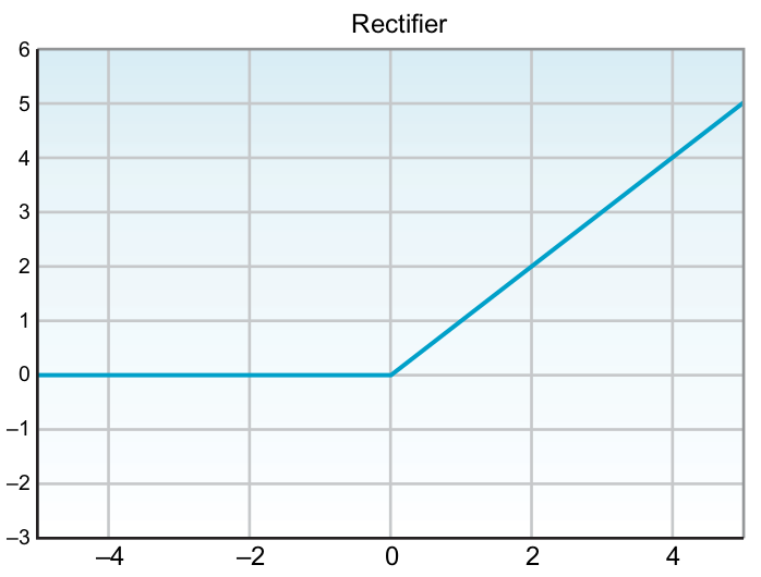
After the transfer function, the summed product of nodes and weights, the activation function will be applied, and the outcome from this process will remain only positive values.
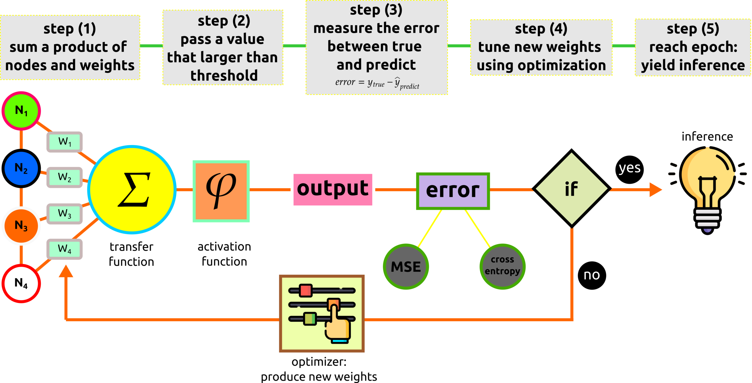
Perceptron Pipeline
misclassify
(non-linear)
Example of Input Features
misclassify
(non-linear)
tabular data
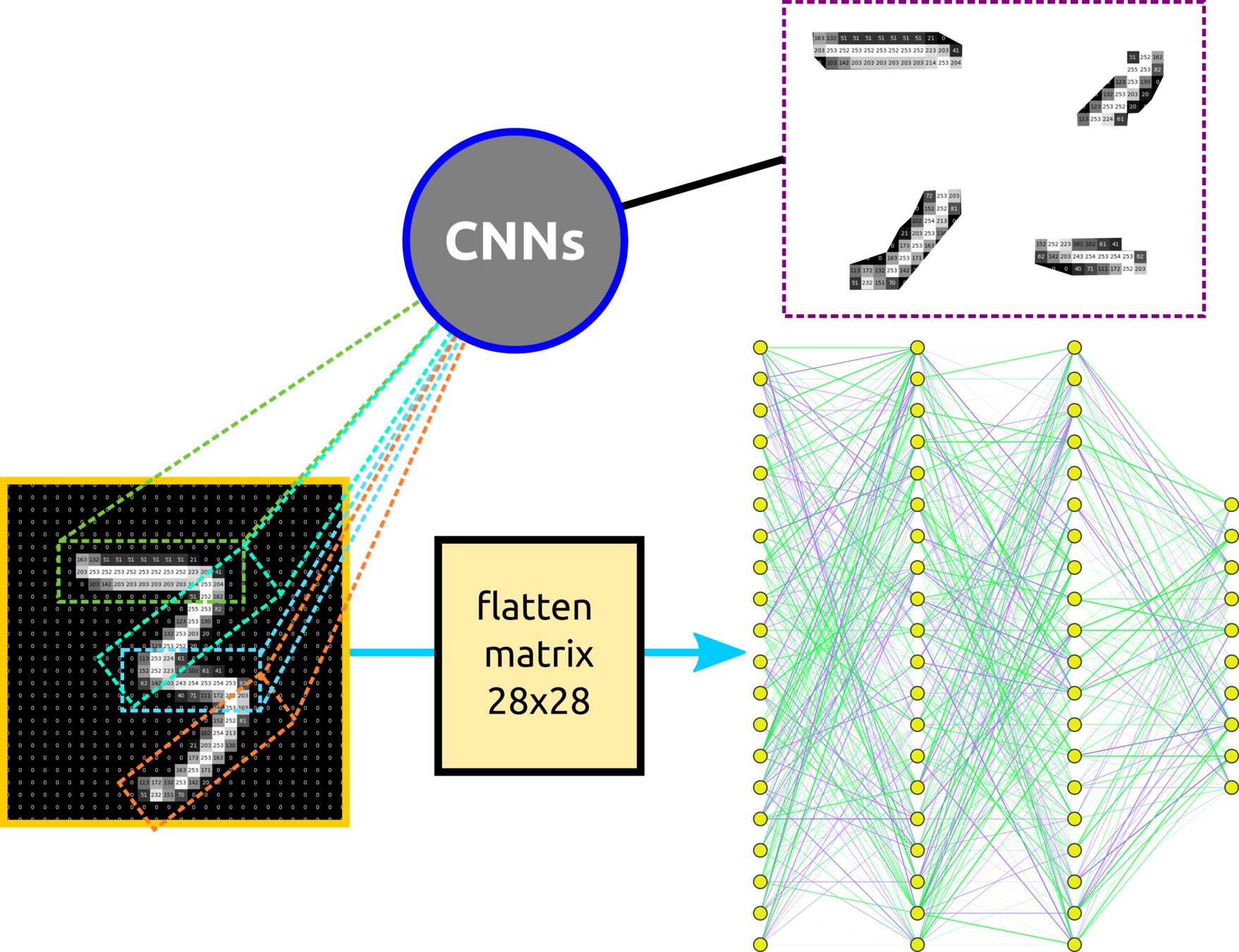
image
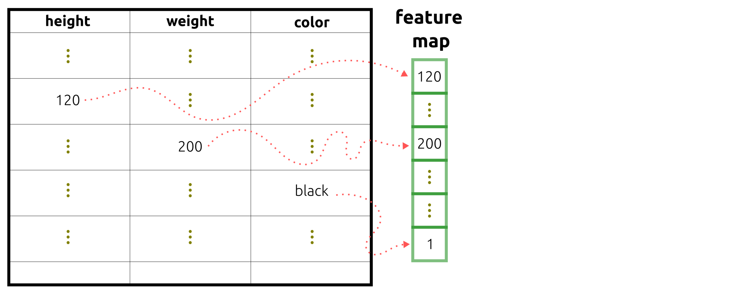
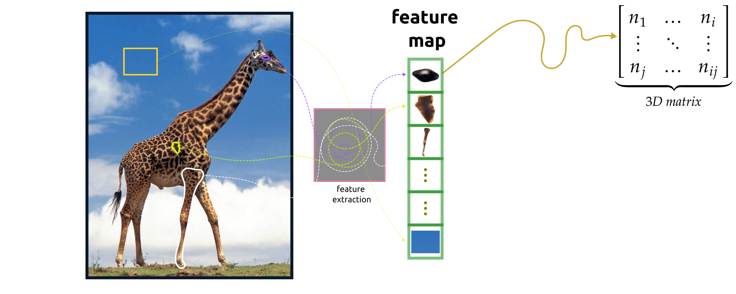
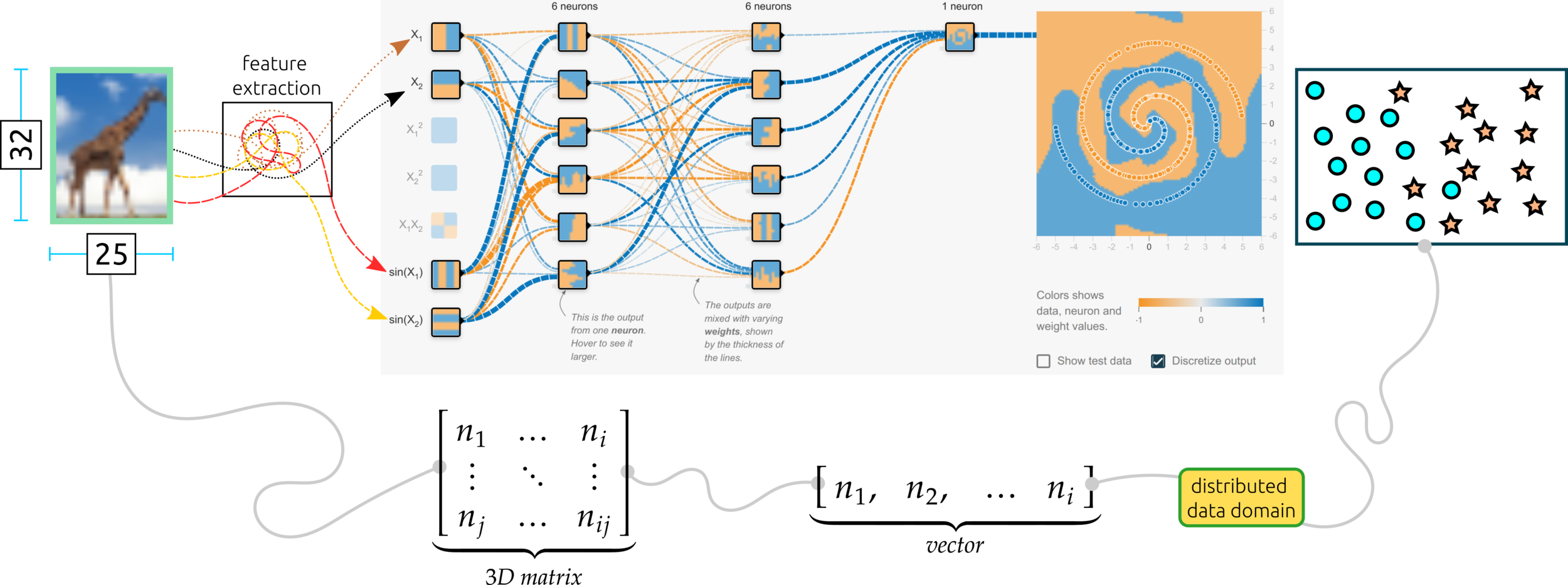
The input data passing to a feature map or multi-nodes can be a vector and matrix. Before this process, hot-encoder or feature extraction is required.
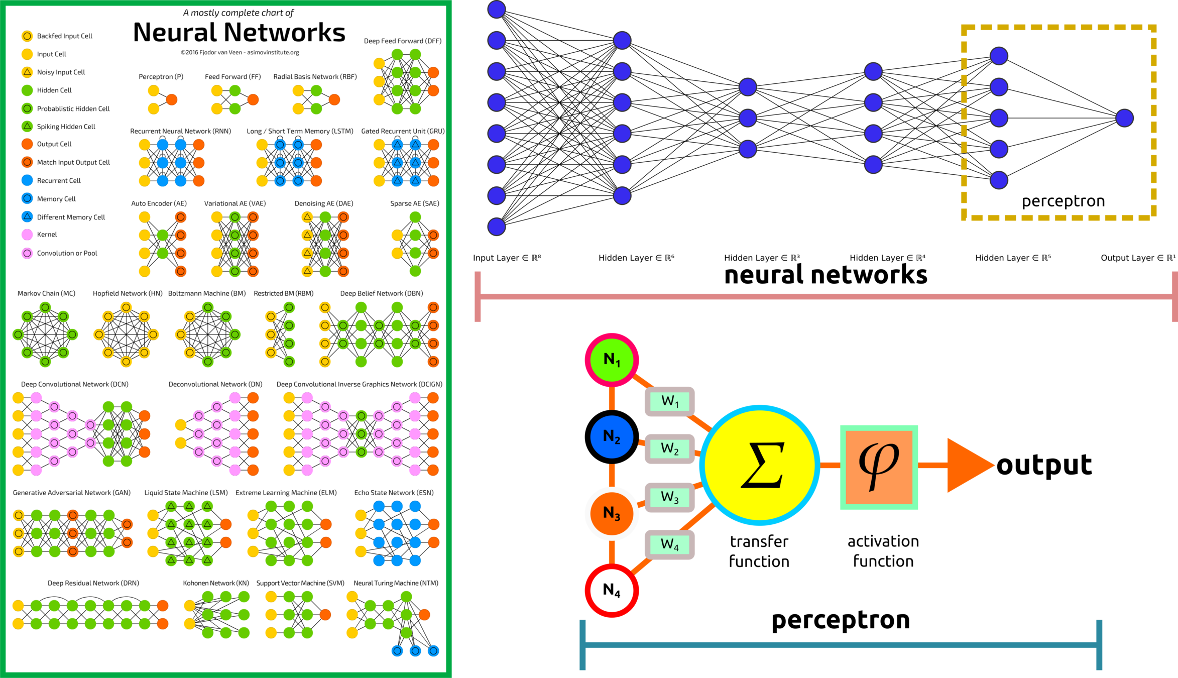
ANN, MLP, and Fully Connected Layer
misclassify
(non-linear)
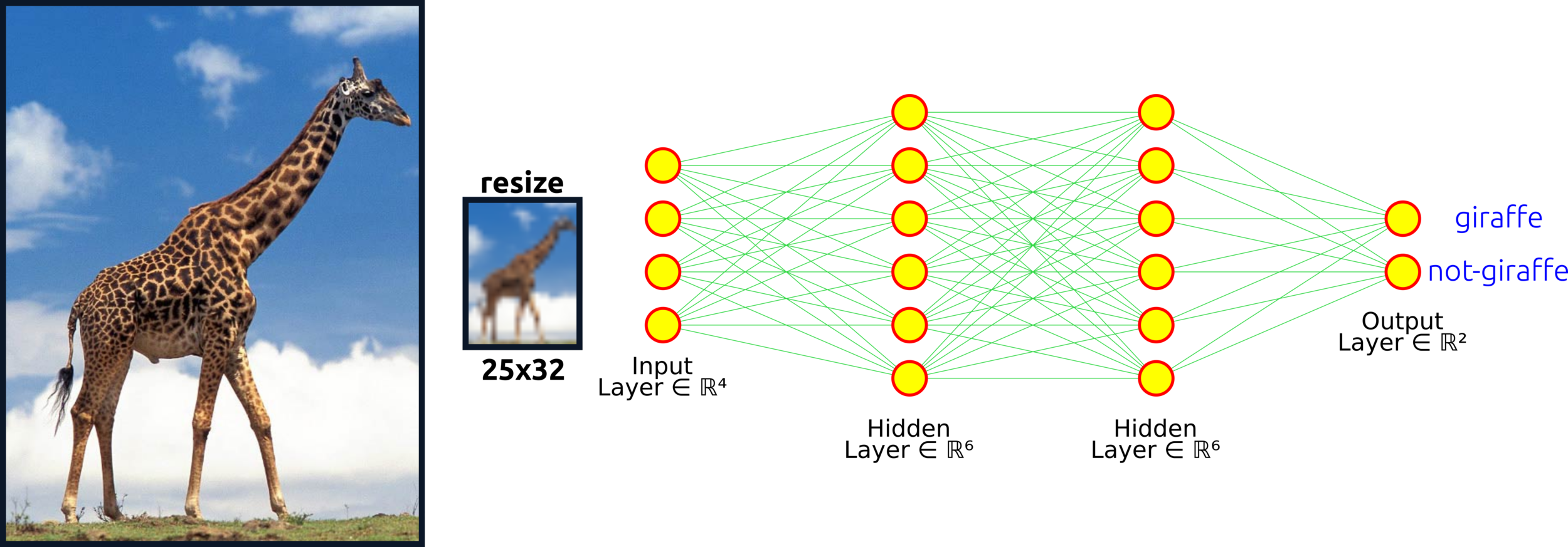
Classic terminology shares several similarities among artificial neural networks (ANN), multilayer perceptron (MLP), and fully connected layers. Those types can represent such as the neural network architecture here.
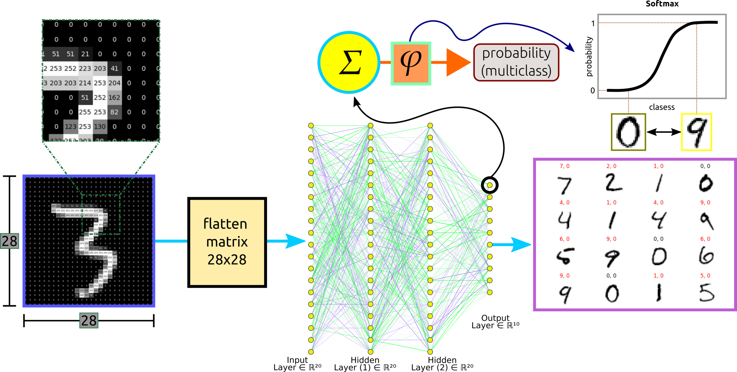
Input layer: one node contains one pixel, so the first layer has 25x32 = 800 pixels. In the case of a complex network, the input layer might be an extracted feature (3D matrix).
input layer
hidden layer
weight
connections
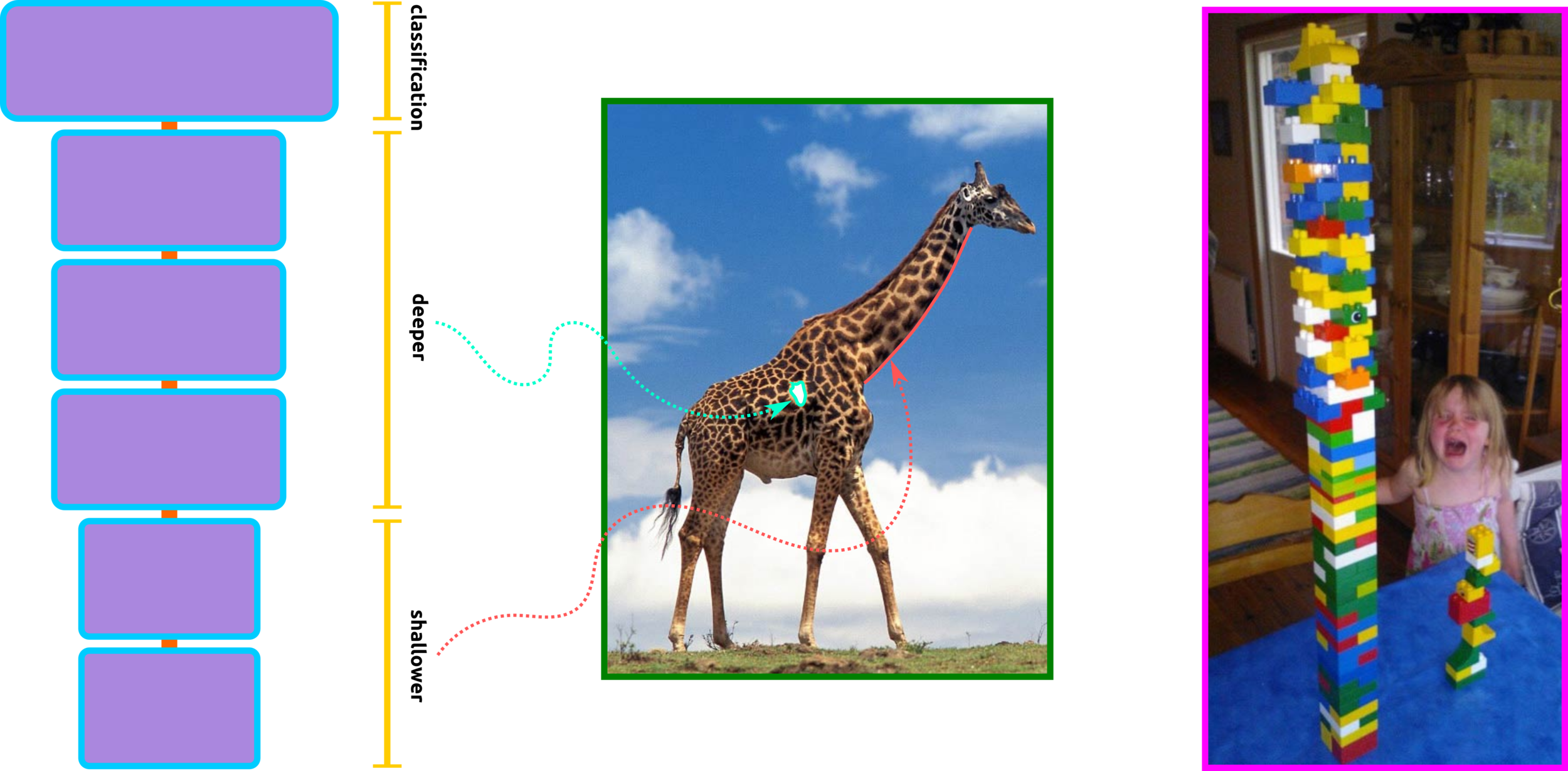
Hidden layer: the first learning process starts from this layer. Increasing nodes and layers here can help the algorithm classify data better. For example, the eye of the giraffe might be extracted from some node in the layer. Keep in mind that adding more nodes and layers will in crease computational cost.
Weight connections: multiple edges connected to nodes among layers are weights in the network algorithm that enhance important features and diminish insignificance features; some nodes might have more weight (useful features) than others (less valuable features).
Output layer: the result from this layer depends on activation functions. If the activation function is regression, the predicted output can be a real value. The output yields probability confidence in the classification problem for probability types in the activation functions.
output layer
Activation Functions
binary
multiclass
hidden layer
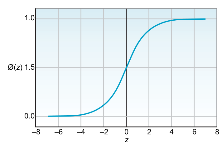
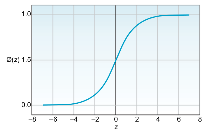
Sigmoid
Softmax
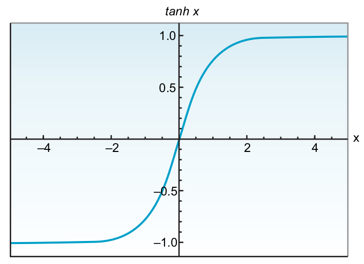
Hyperbolic
tangent
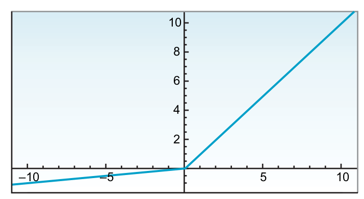
Rectified linear unit
Leaky
Relu
CONVOLUTIONAL NEURAL NETWORKS ARCHITECTURES
Refresh How ML Classifies Images
K-Means
SVM
decision tree
Refresh Data Transformation
In-Depth MLPs
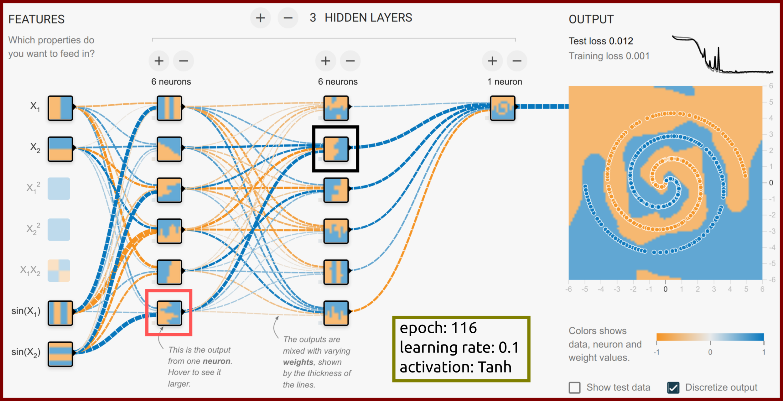
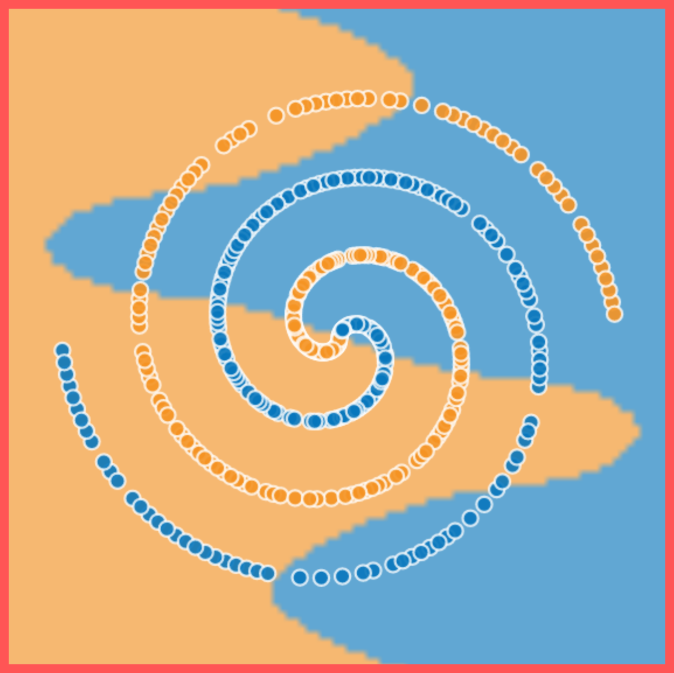
learn a simple feature of the blue data
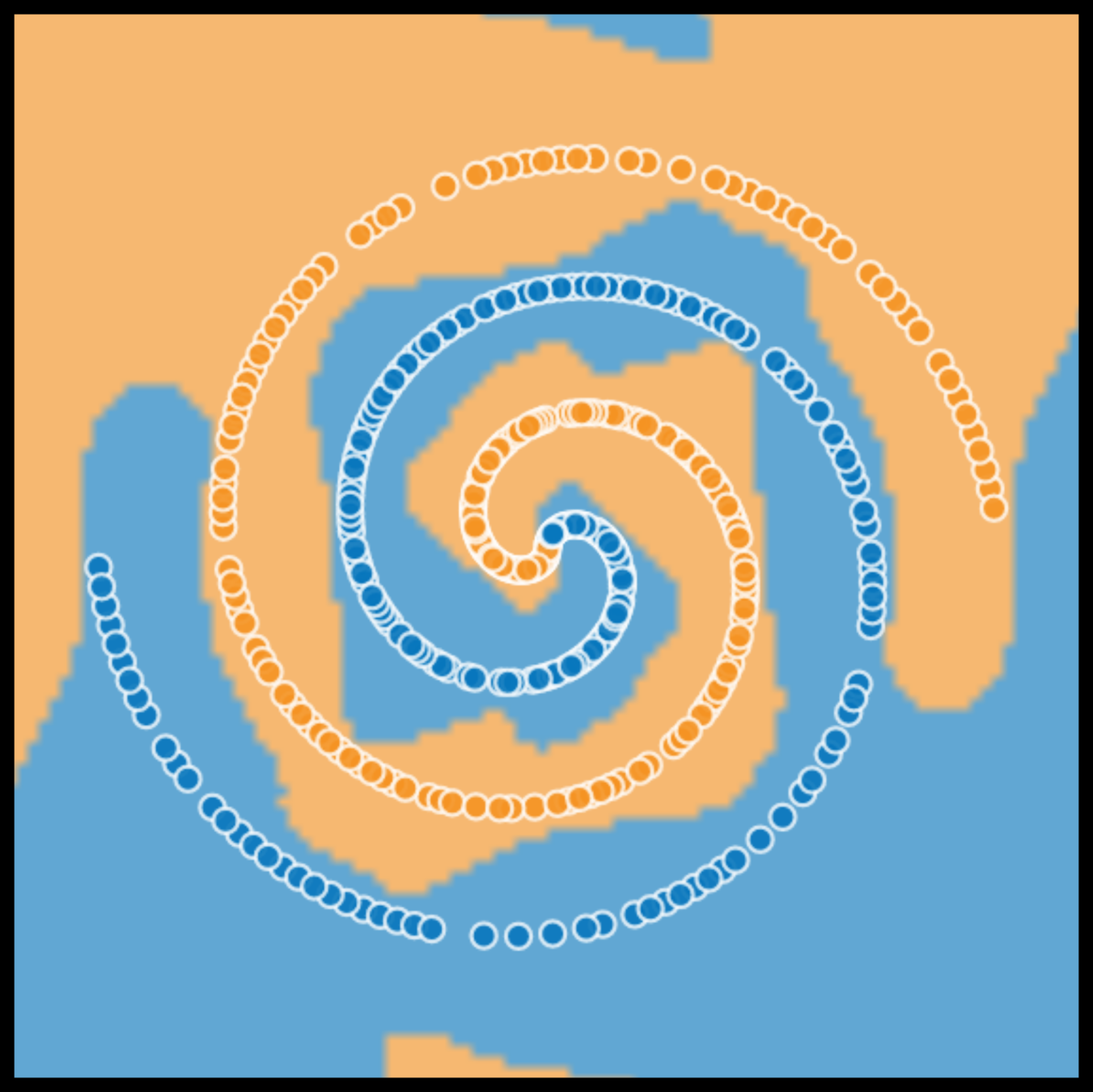
learn more complex feature of the blue plus orange data
Some Thought: In-Depth MLPs
MNIST Classification Using MLPs
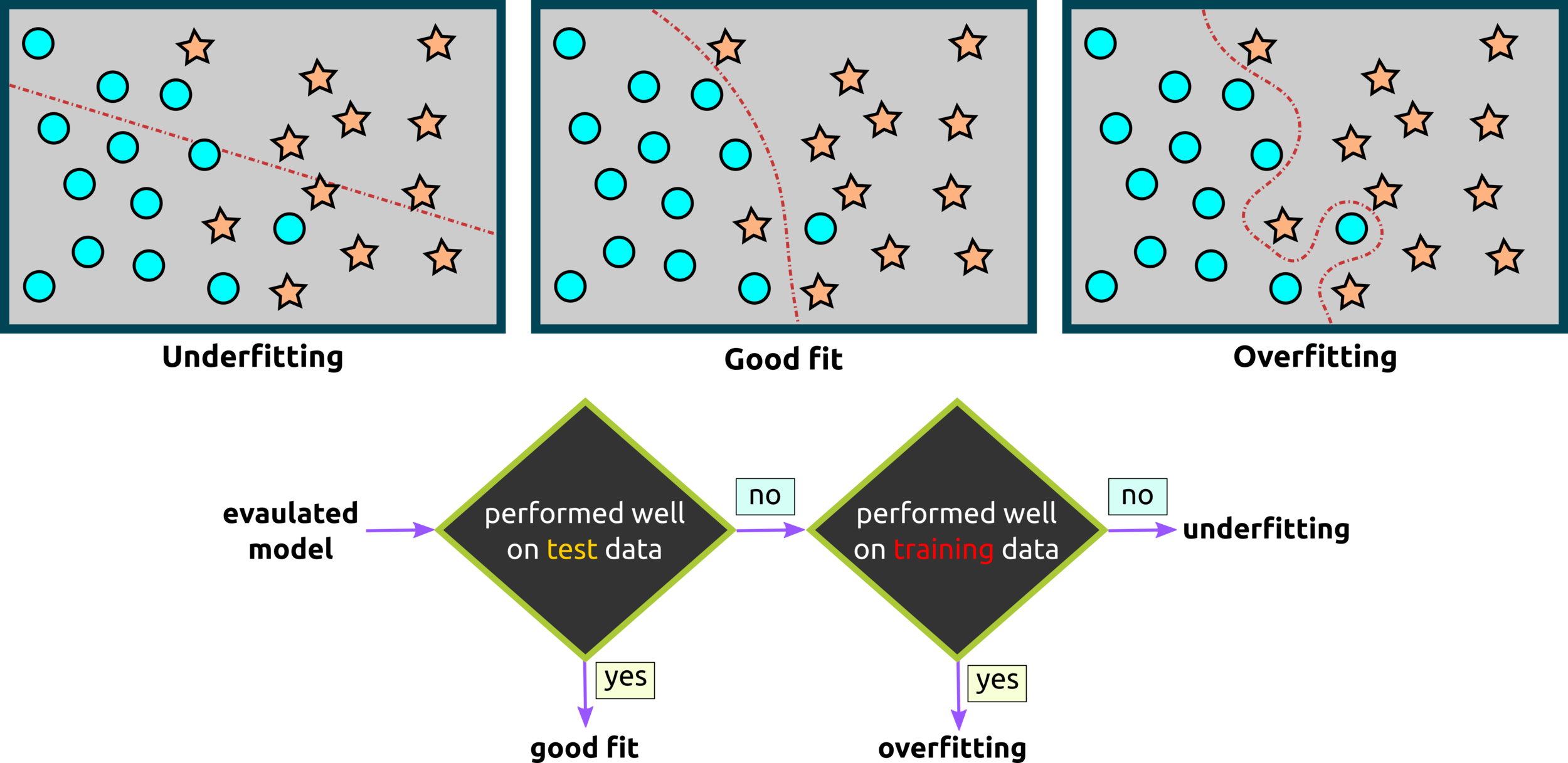
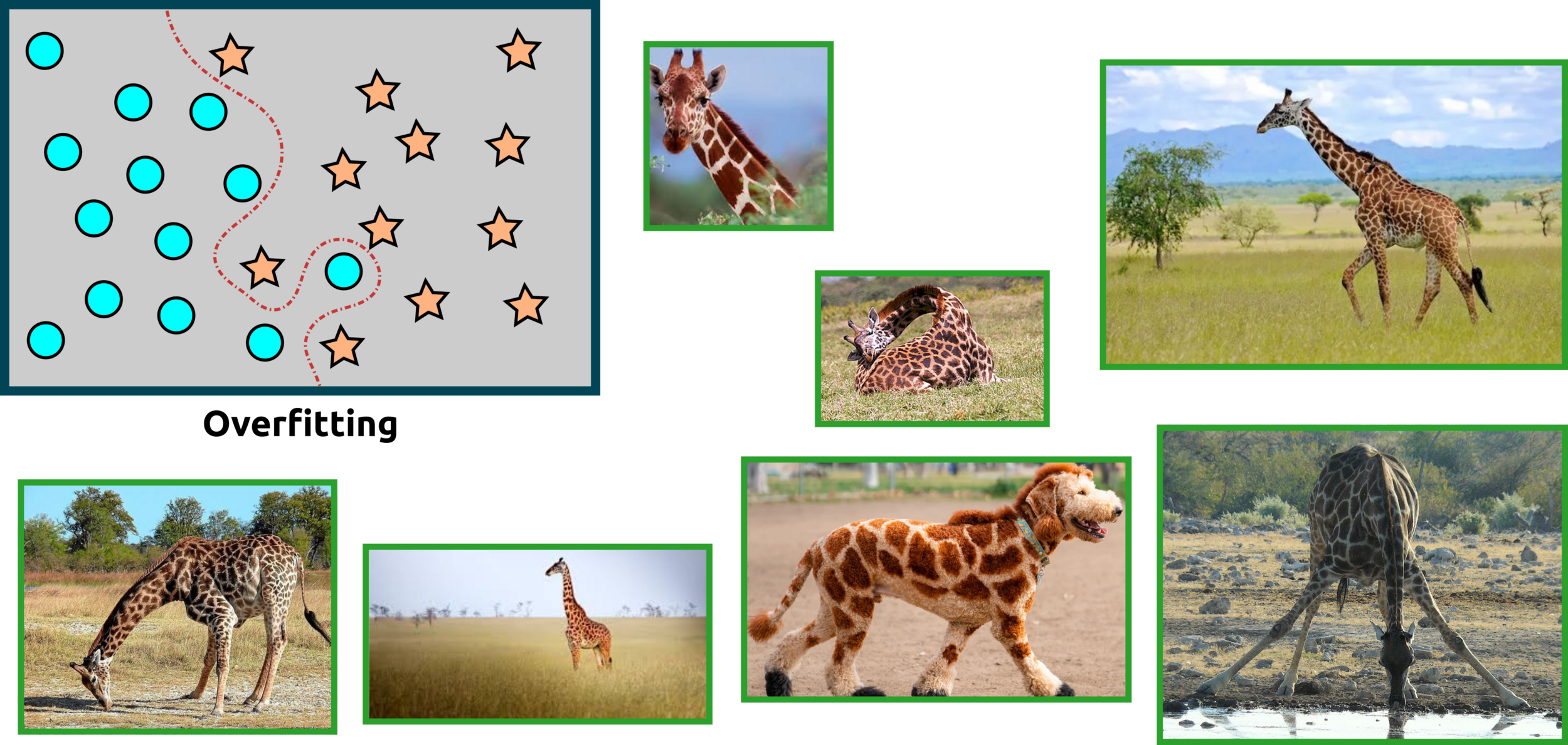
Underfitting - Good Fit - Overfitting
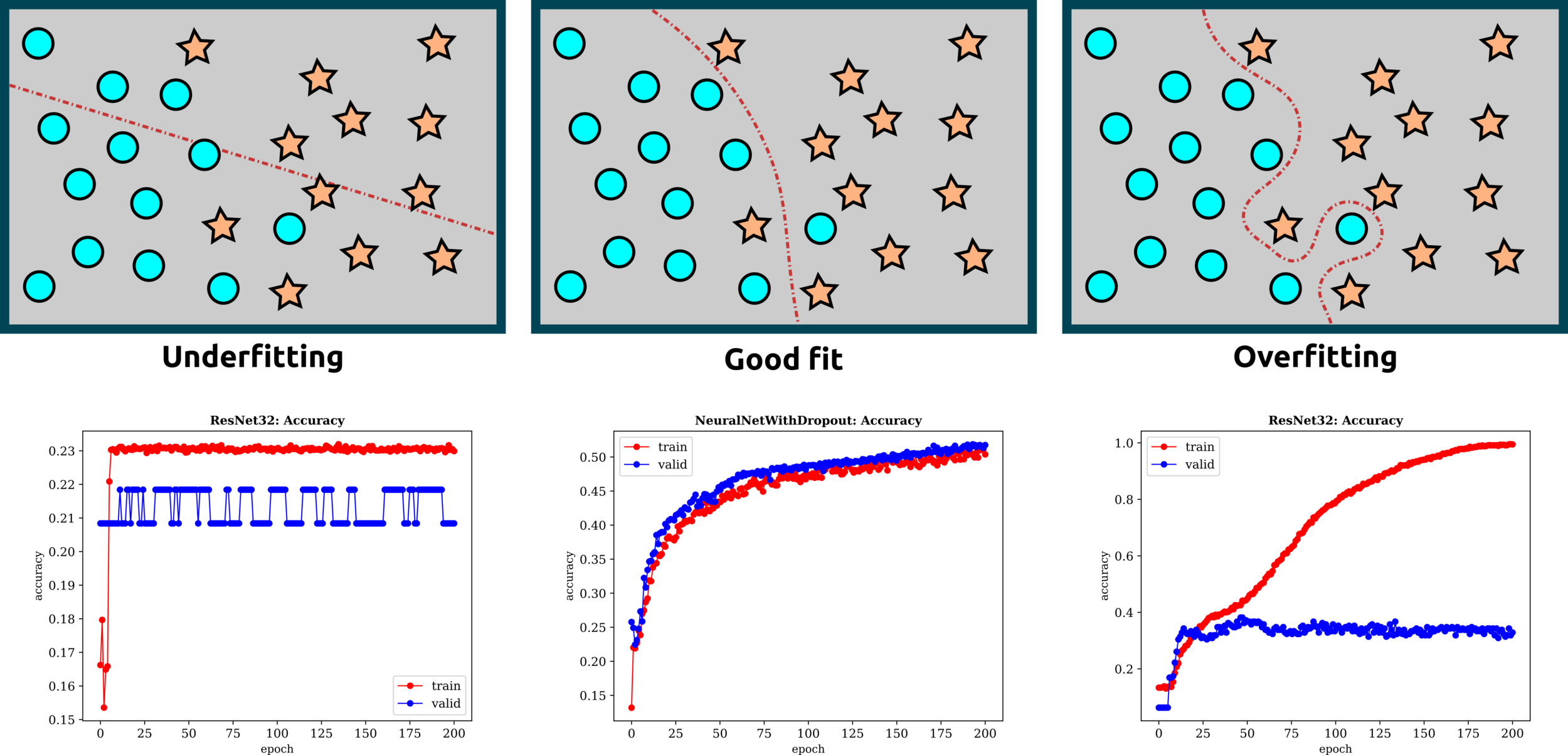
Underfitting - Good Fit - Overfitting: Examples
Some Thoughts: Overfitting
Limitation in MLPs: CNNs Outshine MLPs
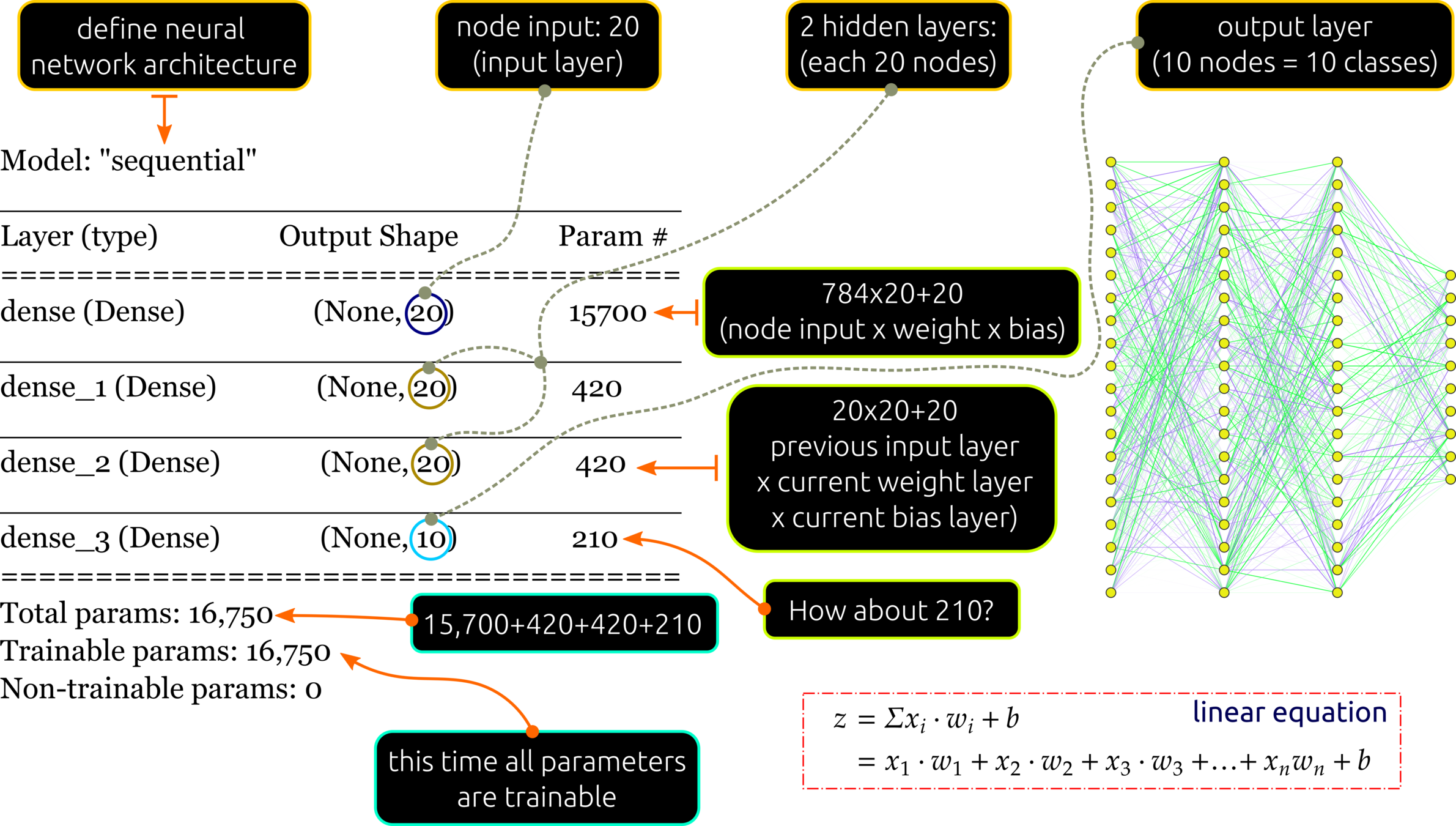
To avoid exhausting computation, such as this simple networks connected 70 nodes with a total of 16,750 parameters for the fully connected layer. CNNs are designed to overcome this problem by extracting some features to train so-called locally connected neural net.
Neural Network Components
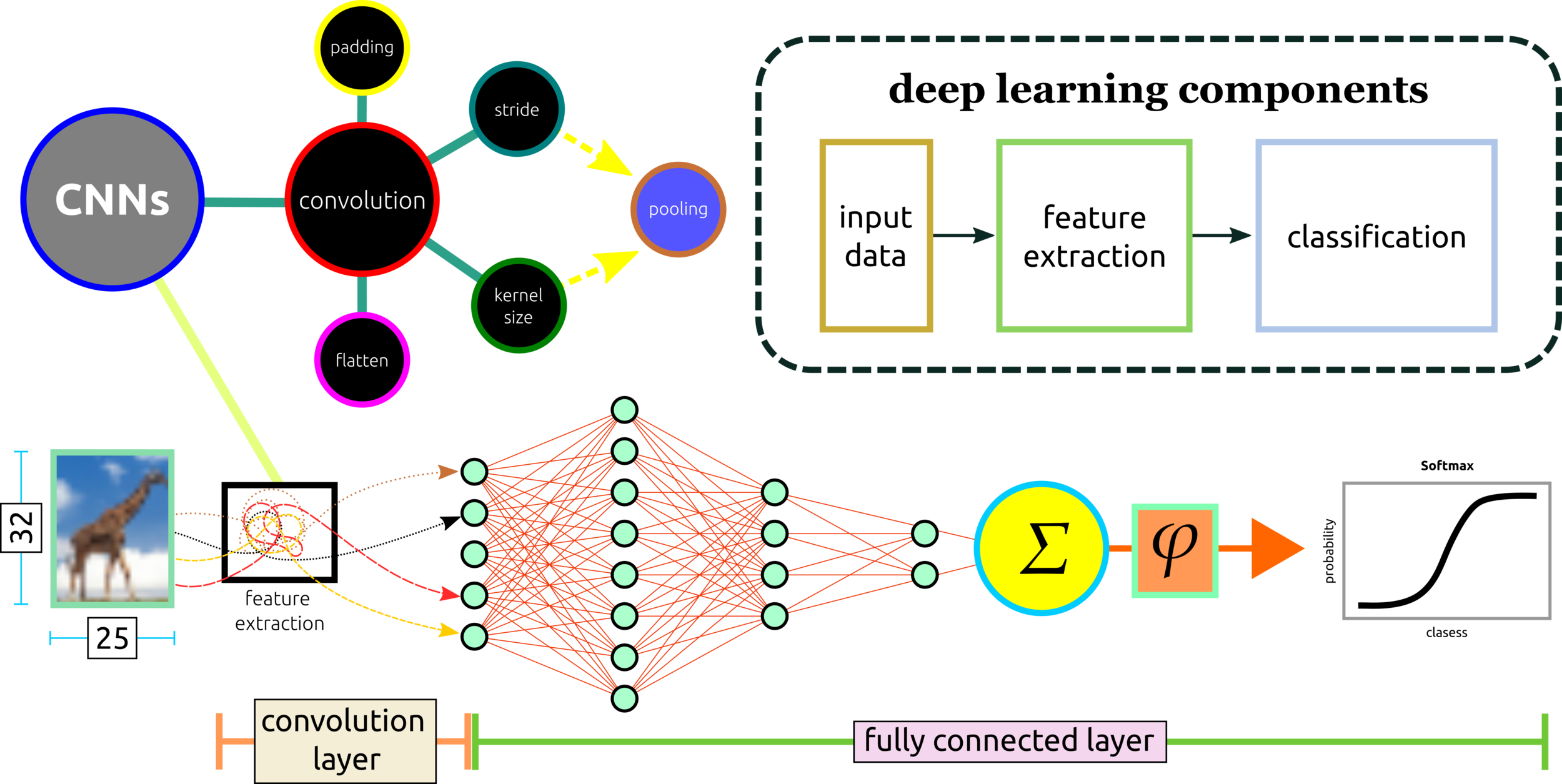
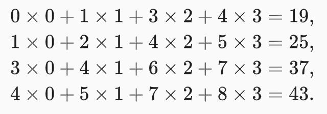
Convolution

Pooling, Stride, Pad, Kernel Size

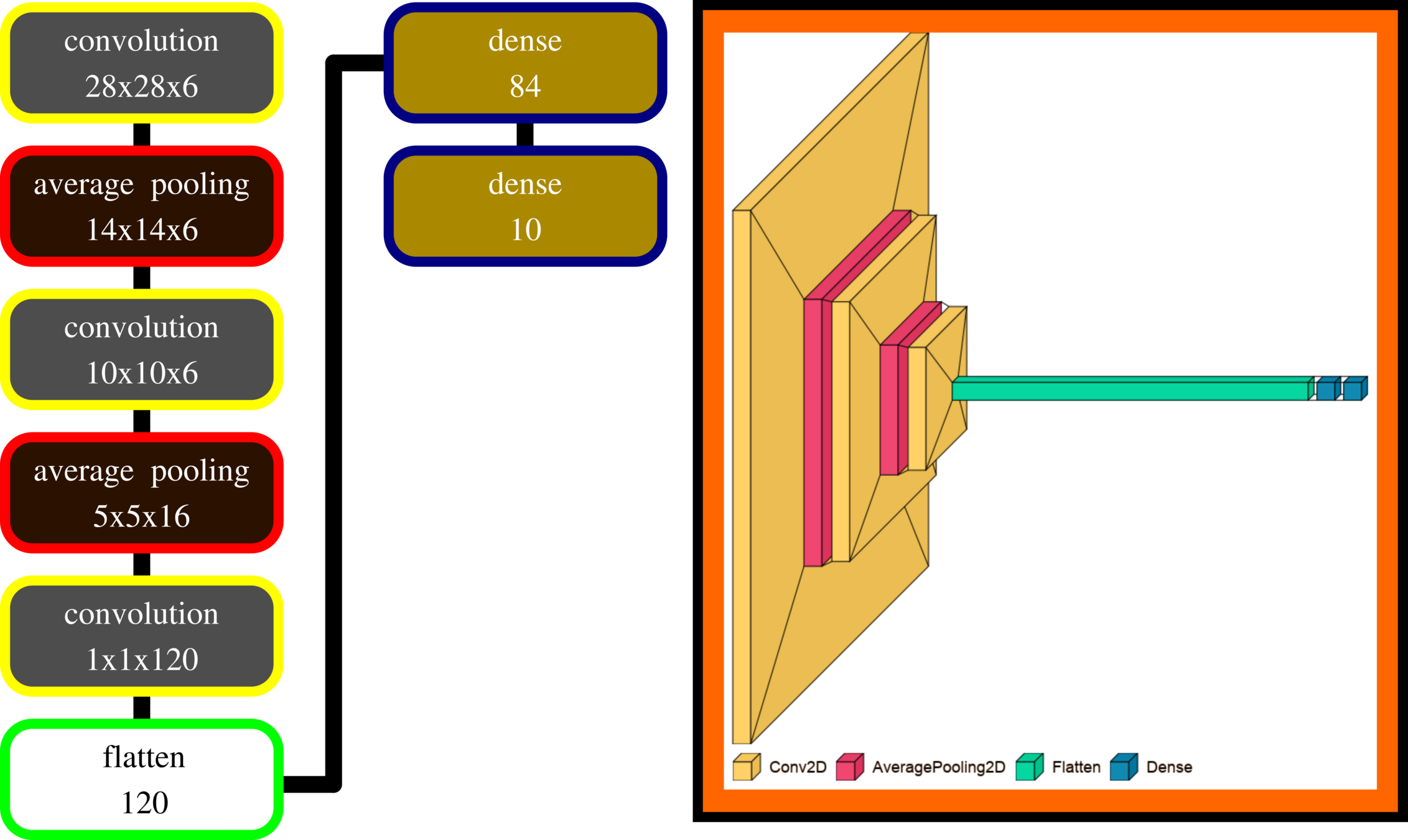
LeNet-5 (MNIST)
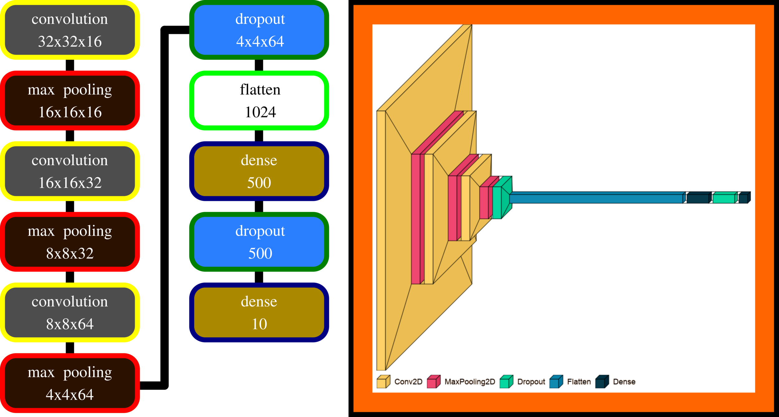
AlexNet (CIFAR-10)
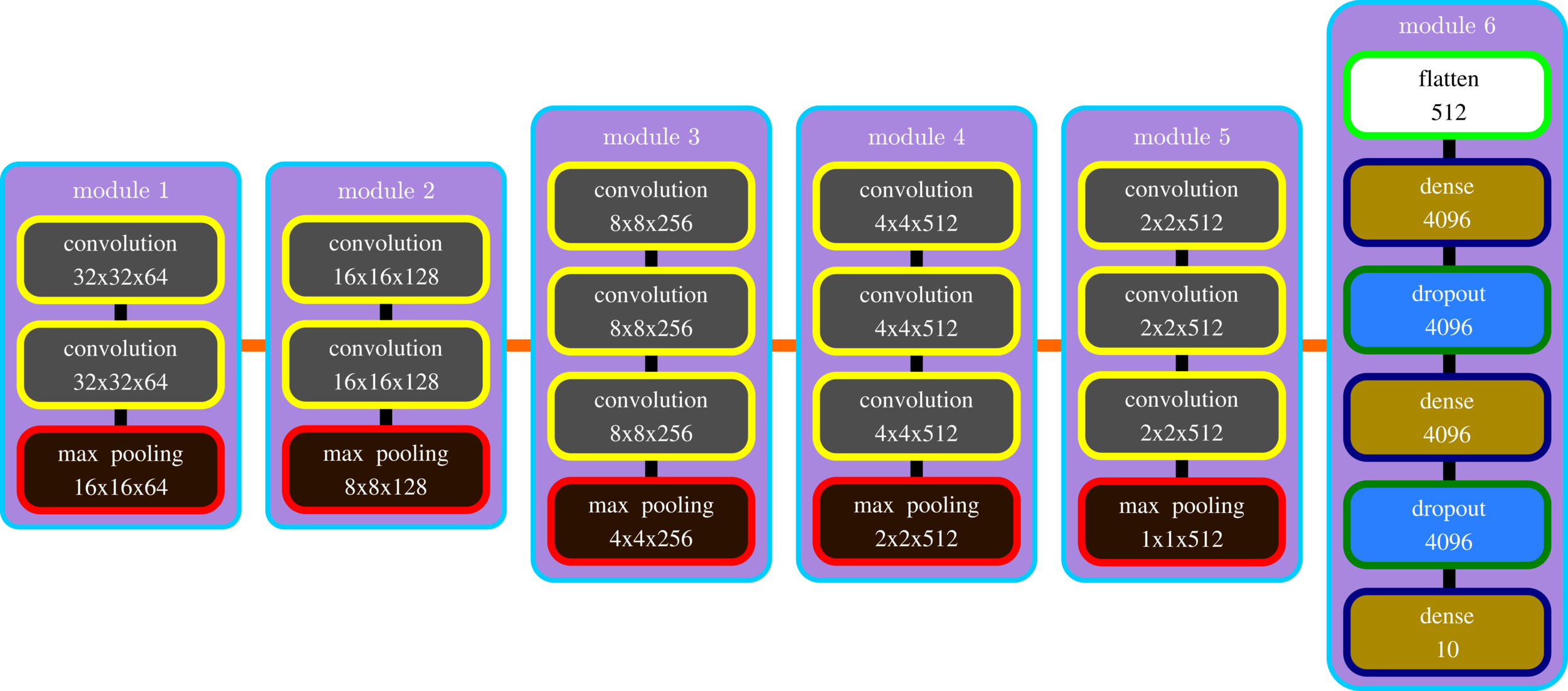
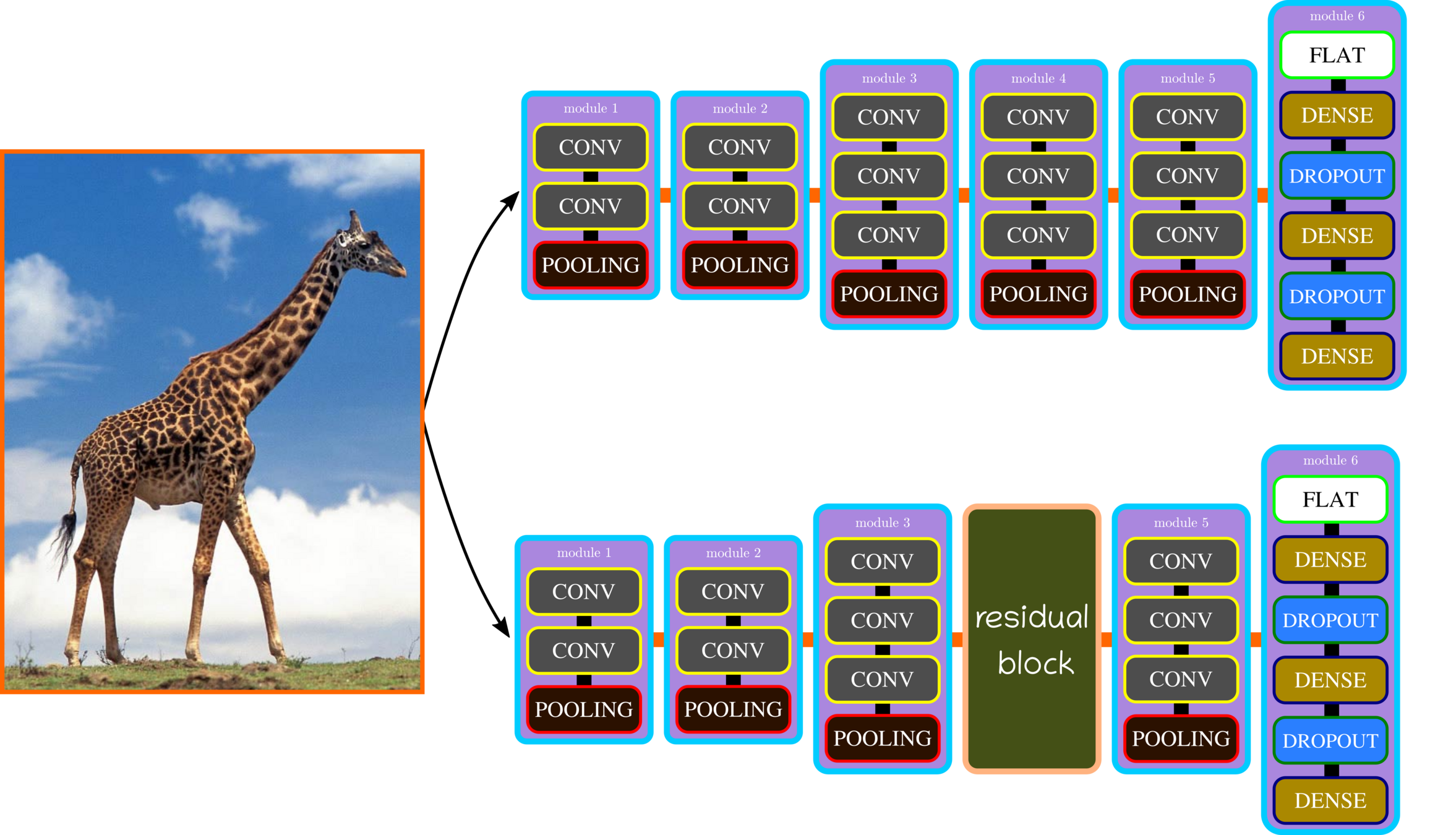
VGG 16 (CIFAR-10)
block networks

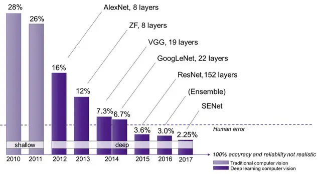
To Sum Up, the Deeper - the Smarter Net?
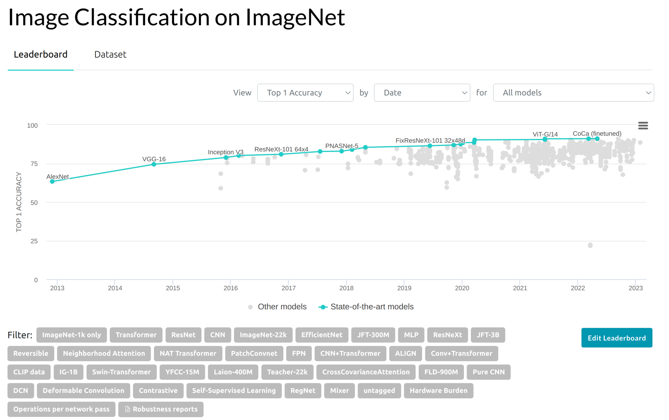
Beyond VGGNet
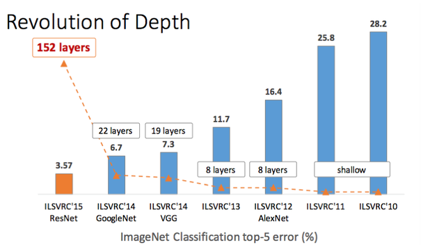
Beyond VGGNet
ADVANCED NEURAL NETWORK
ARCHITECTURES
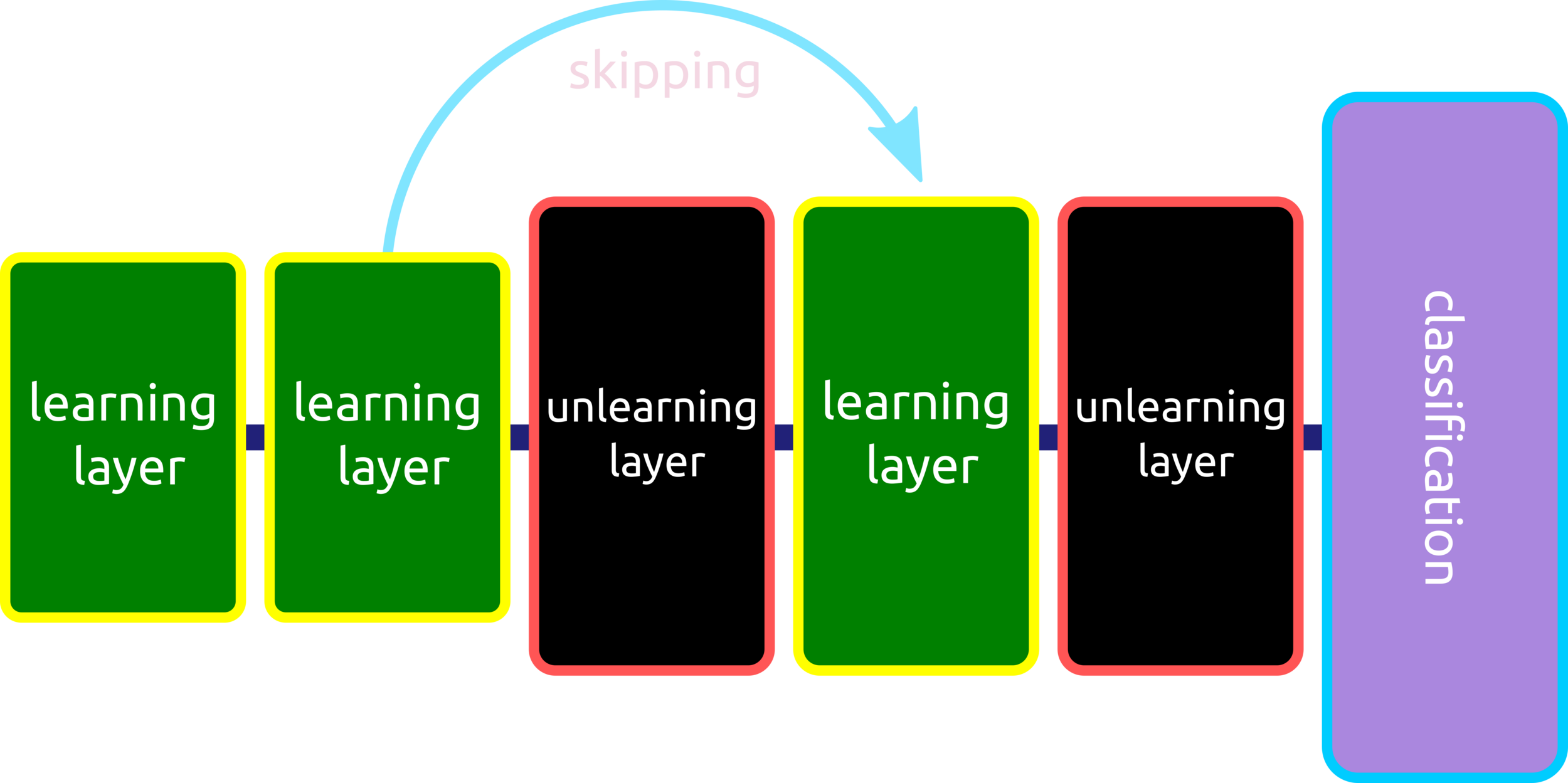
Residual Networks (ResNets)
The deeper layers are not the more intelligent neural networks. ResNets are designed to overcome this pitfall by using skipped layers to avoid vanishing gradients. This technique can skip duplicated unlearning layers and stack learning layers.
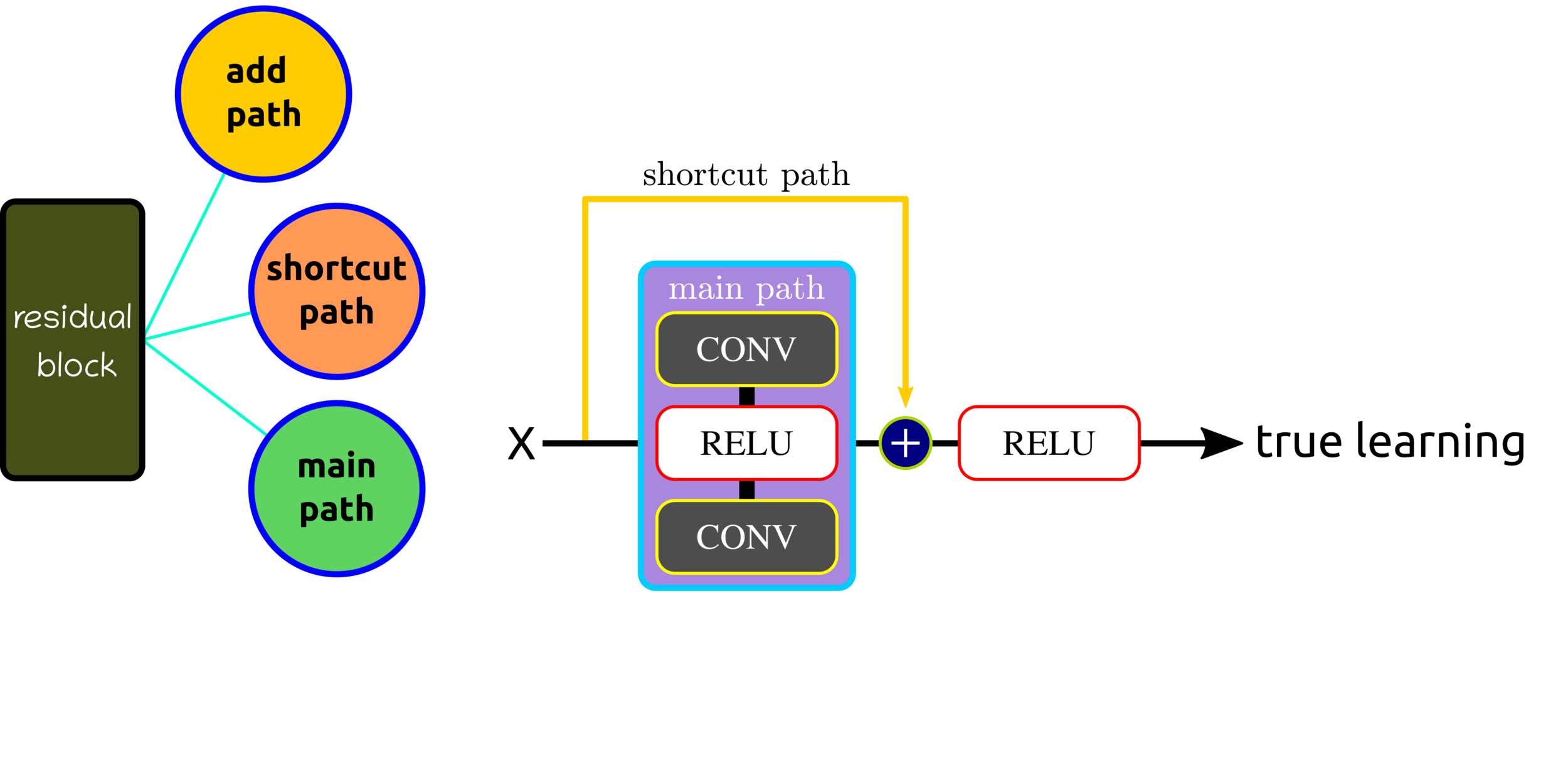
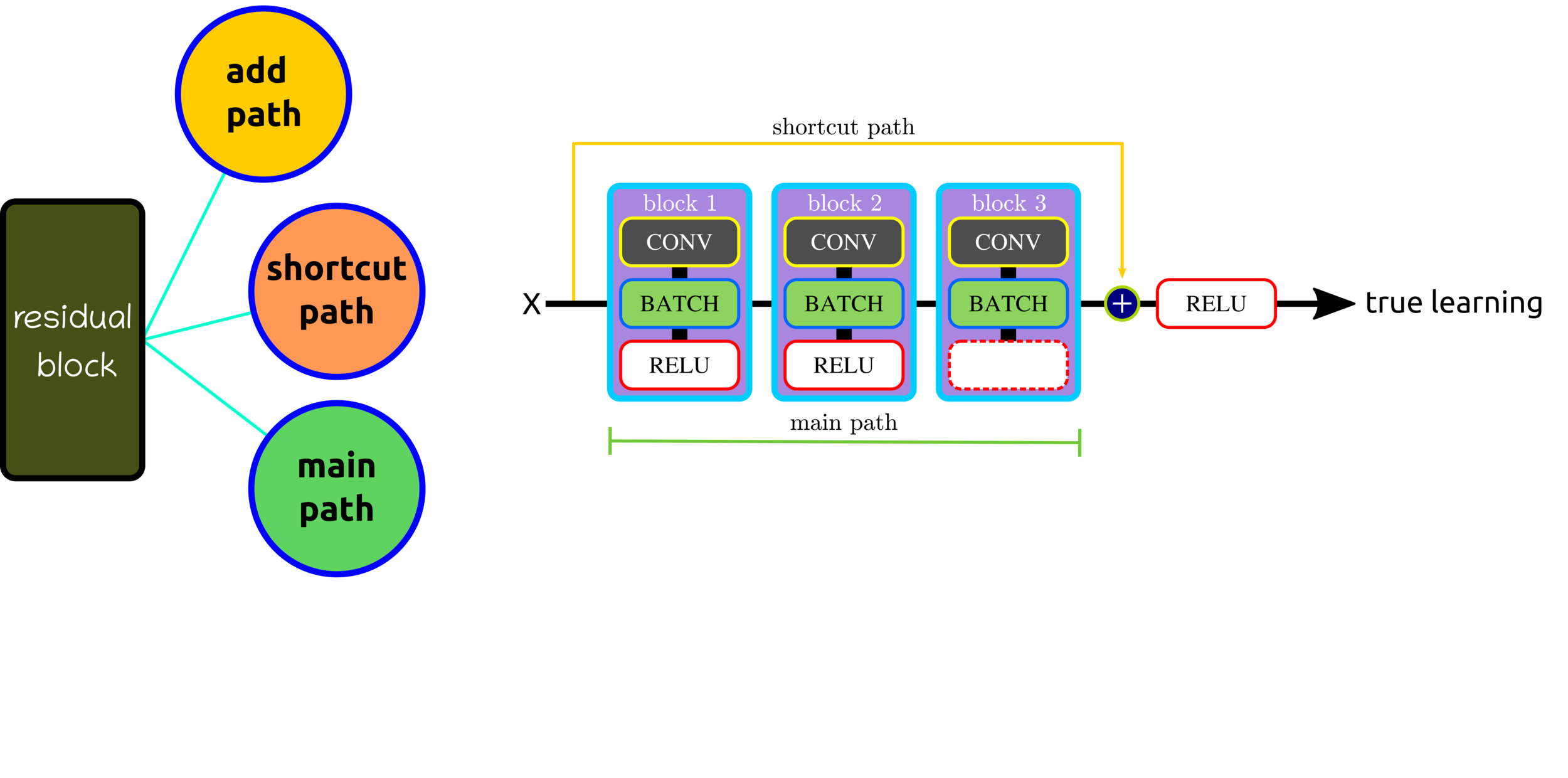
Residual Block Components
Residual Block: Control Volume Dimension
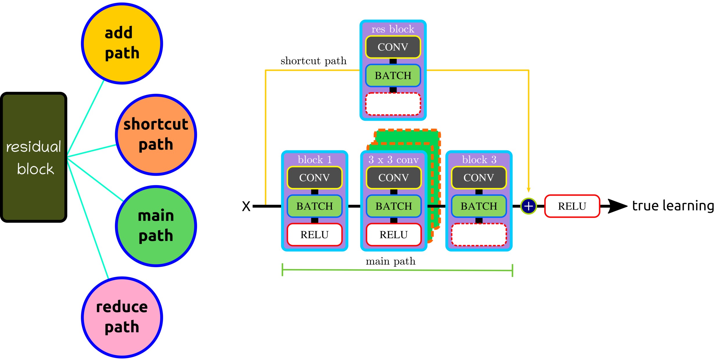
Residual Block: Reduce Shortcut
ResNet (Layers)
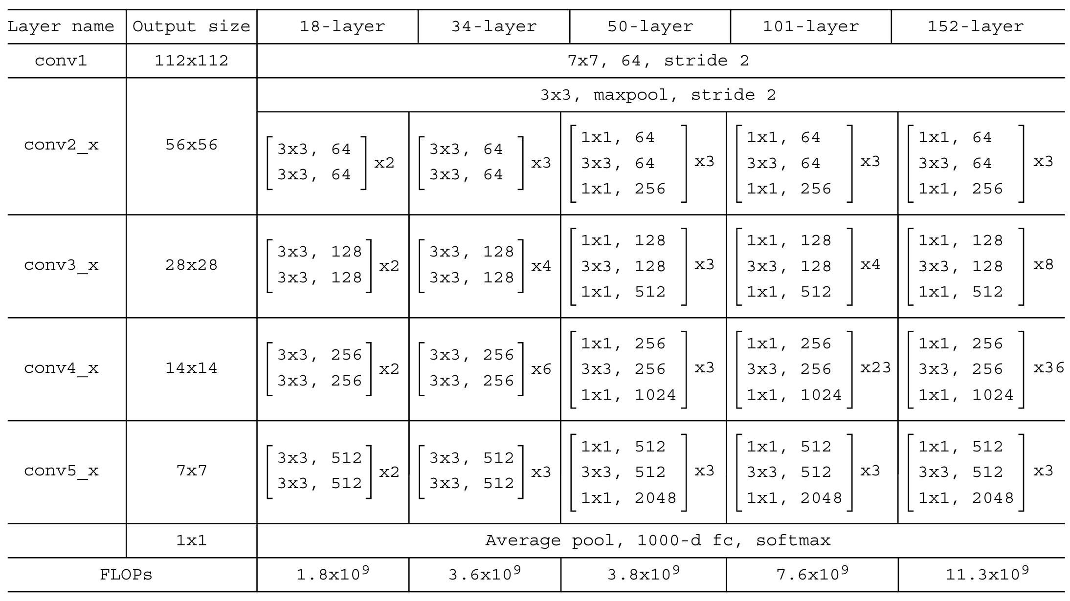
IMAGE SEGMENTATION
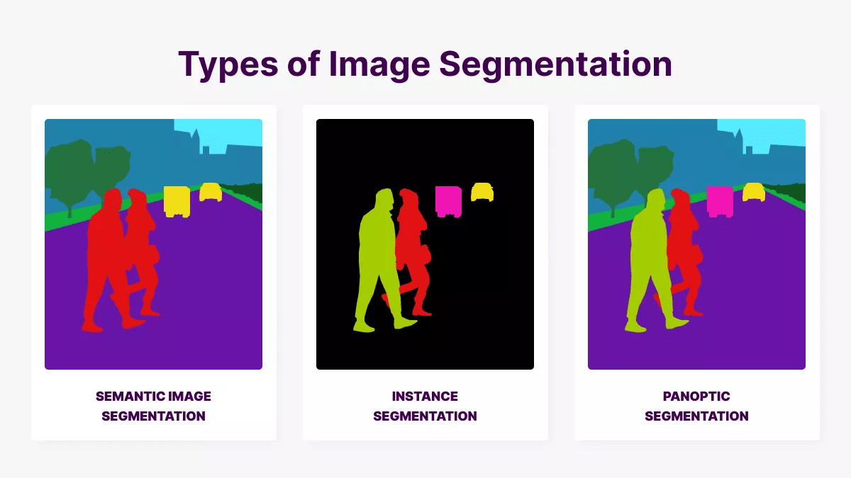
Set of Pixel vs Pixel Classification
Image Classification
Image Segmentation
Vision Transformers

02_DL_23
By pongthep


