2307588
FALL 2021
MACHINE LEARNING
FOR GEOSCIENCES
calendar
Aug
Sept
Oct
Nov
Dec
12 first-day class
midterm
Oct 07
CH 1
CH 1
no class
CH 4
CH 4
CH 3
CH 2
final
Dec 02
no class
CH 5
CH 5
CH 6
CH 7
CH 7
CH 7
ITINERARY (MIDTERM)
MIDTERM PROJECT
ITINERARY (FINAL)
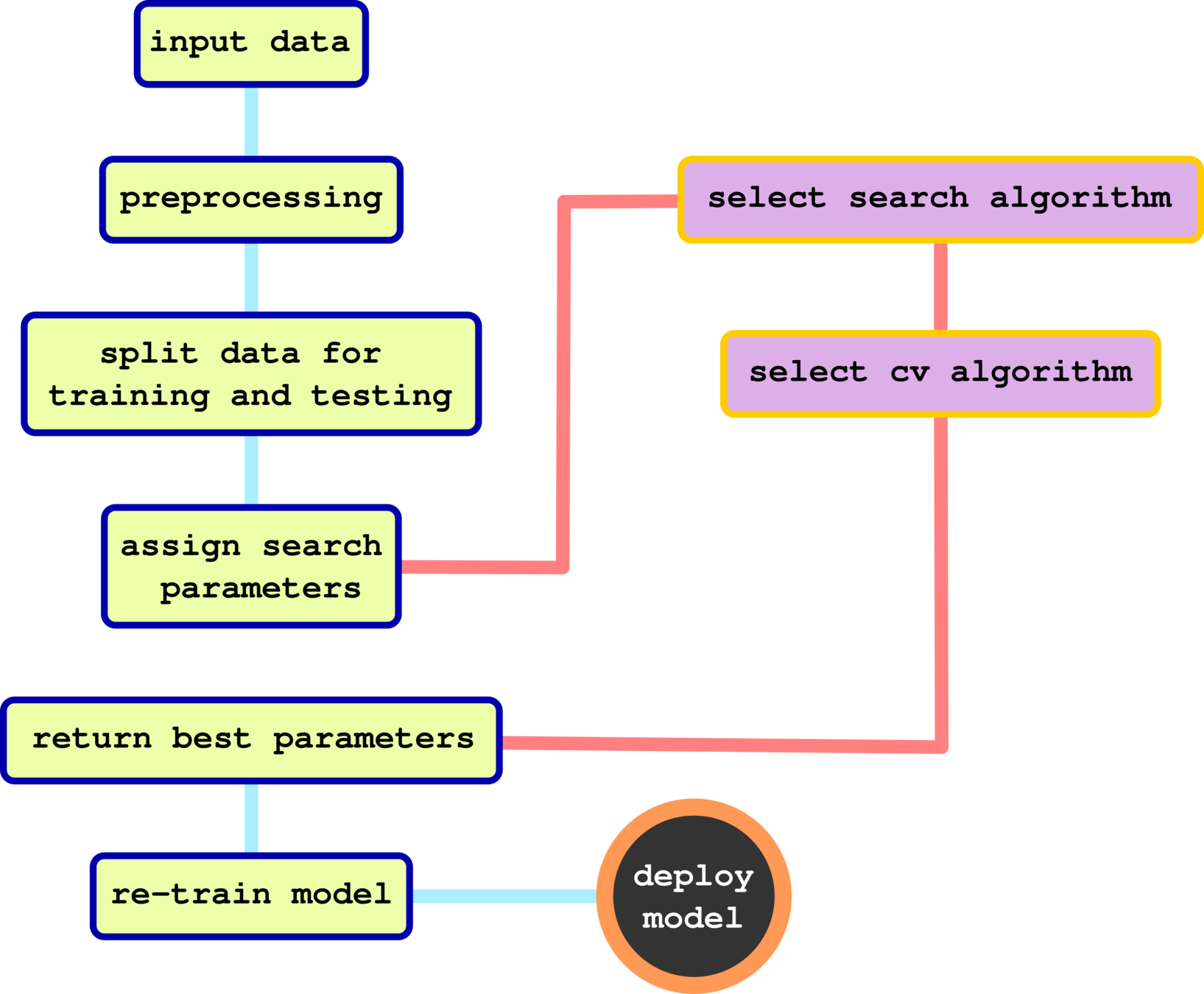
HYPERPARAMETER TUNING
CH: 6
GREDIENT BOOSTED DECISION TREES
CH: 5
HANDON FINAL PROJECT
GAUSSIAN PROCESS REGRESSION
CH: 7
ML and DL for Geosciences
MACHINE LEARNING
AUTOMATIC ML
class 2307588
class 2307589
DEEP
LEARNING
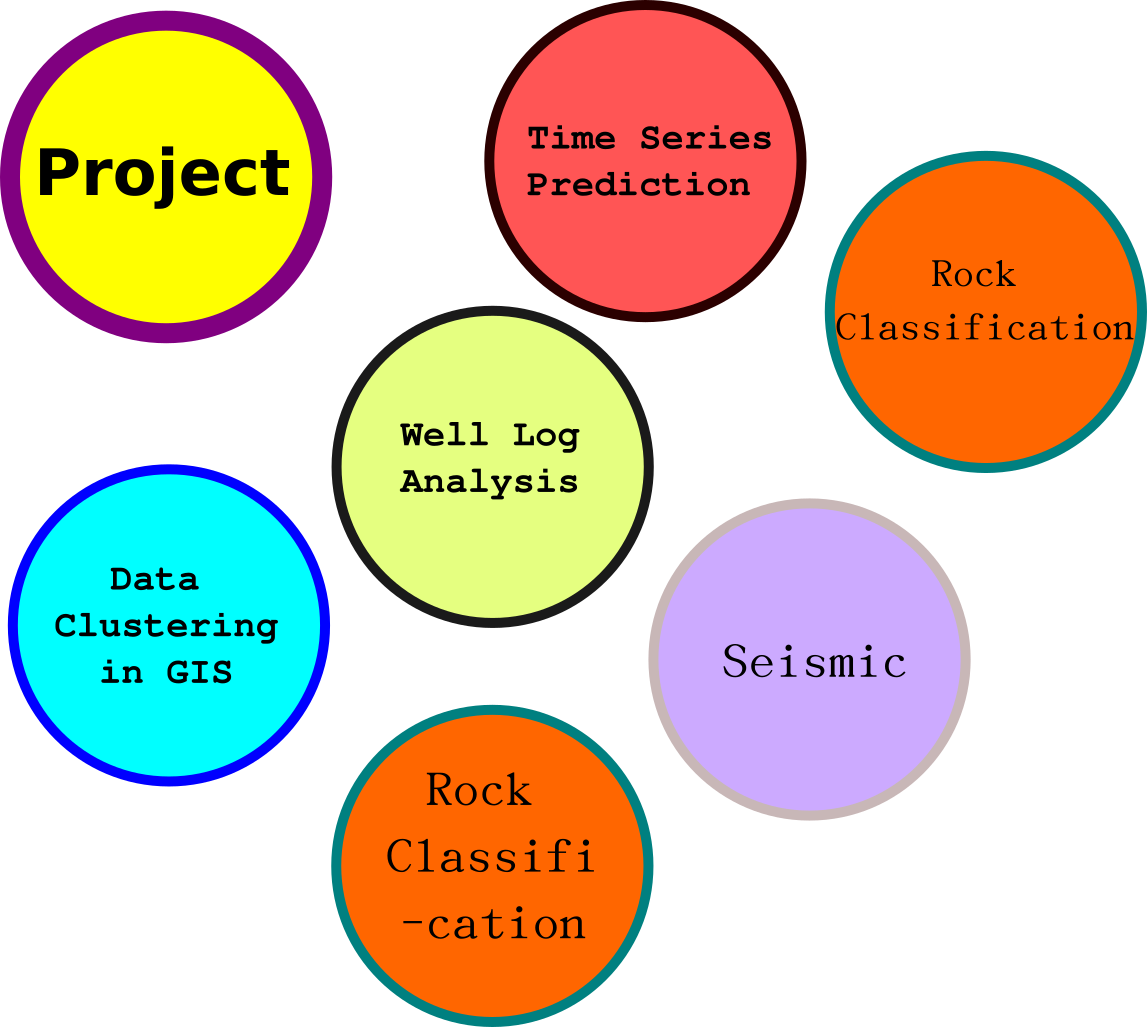

Time Series Prediction
Well Log Analysis
Data
Clustering
in GIS
Microscope/fossils
Seismic
Rock
Classification


Grading Policy
midterm 30%
final 60%


RULES:
project based learning
bonus 10%
-
always on time
-
behave like sit-in class
-
absent more than 2 times, you will lose bonus score
-
always on camera (is a must)...I want to observe that you didn't sleep during class
-
no phone during class
-
please stay at home or properly studied environment... not coffee shop, beach, restaurant...keep in mind that you have responsibility to answer your friends and instructor's questions
-
dress properly
Ecosystem


Installations
Classic Equation

F = M \times A + (\alpha 1 + \beta 1)

neuron networks
Modern Equation
the network equations that human can program
a computer to know how to learn
artificial intelligence
machine learning
deep learning
AutoML
supervised learning
unsupervised learning
A Broader Family of ML Methods
Supervised Learning vs Unsupervised Learning
Classifcation
Latent Space in ML
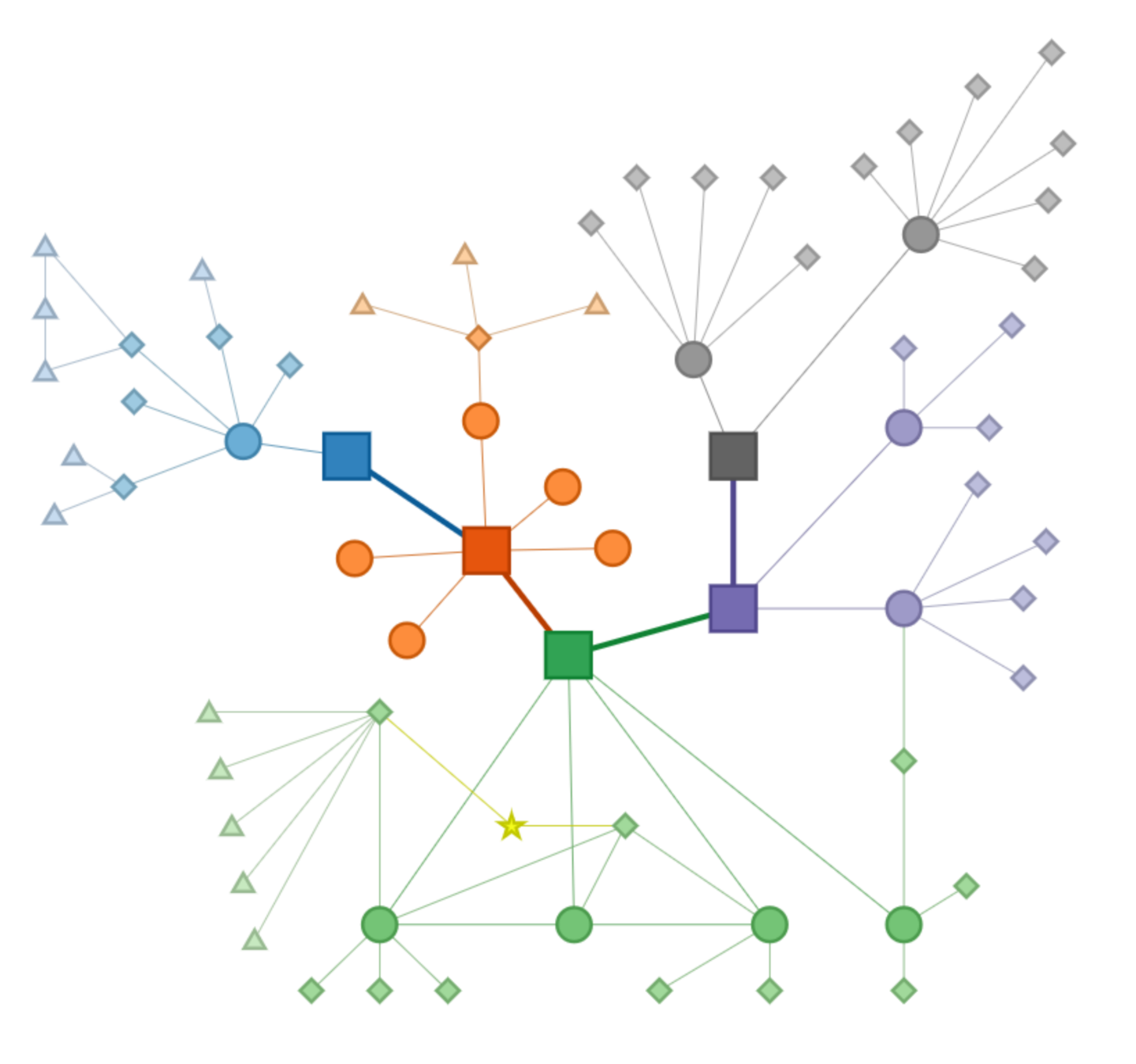
Course Overview
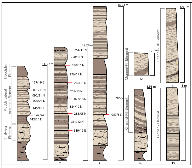
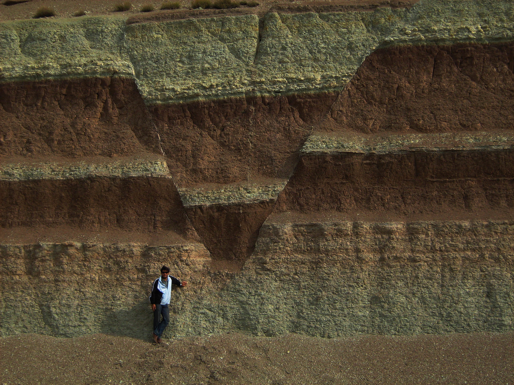
The figures show that the intervals contain sequence stratigraphy of fluvial environment exposed to the surface. Geoscientists can interpret the rocks based on colors, gain sizes, and minerals. So how can we obtain the subsurface information?


In order to obtain that information, geoscientists deploy wirelines into a borehole to measure a formation property. Each rock layer contained different kinds of minerals that possess distinguishable characteristics. However, their properties are not discrete, which requires tremendous works to classify. Here, we will follow the SEG competition 2016 to study ML/AutoML workflow to create a robotized framework of petrophysical analysis.
CH 1: INTRODUCTORY PYTHON
Introductory Python
variables and assignment
>>> a = 10
>>> a
>>> 10
Value 10 is assigned as "=" assignment operator into variable a, and variable a will be stored value 10 in memory space in the computer. When compiling variable a, the program will return value of 10.
update variables and re-assignment
>>> a = a + 2
>>> a
>>>
Let us try to modify the variable that previously stores value 10 in the memory allocation, and this time add a new value (2) into the previous variable a. What is the outcome? All variables and values are input on the right-hand side of this code snipped, and the left-hand side is output stored in the assigned variable named a.
check your understanding
>>> a = a + 4
>>> b = a + 3
>>> a
>>> b
Think about the result and try to explain what variable a and b has been stored.
What is binary?
Did you know? Computer uses the number only 0 and 1 to computerize
Data Types in Python
string
tuple
set
dictionary
numpy array
data

structure
class
and
object
list
matrix
vector
numeric precision
float
integer
complex
bit (byte)
If Statement and For Loop
A > 80
70 < B <= 80
60 < C <= 70
50 < D <= 60
F <= 50
score = 67

if score > 80:
  print('your grade is A')
score = [45, 78, 7, 66, 89]
for i in score:
if i > 80:
print('your score is A')
create for loops with statement conditions to compute the average score of this data.
score = [34, 55, 67, 78, 99, 100, 45, 35.9, 88.45, 89]
Built-In Function and Defining Function
Try to plot cosine and sine functions
Indexing and Row-Column-Major Order

To access element in Python, we need to understand the reference of data position (indexing) and direction to reach the data (row-column-major order). Indexing in Python refers to the position of the memory allocation. By default (Python), it counts the data from "0" and increasing by one. To optimize the speed of accessing element in Python, we should reach the data in row-column major.

row-column-major order
indexing
(2-D)
\mathbf{a_{0, 0}}
\mathbf{a_{0, 1}}
\mathbf{a_{0, 2}}
\mathbf{a_{0, 3}}
\mathbf{a_{1, 0}}
\mathbf{a_{2, 0}}
\mathbf{a_{3, 0}}
\mathbf{a_{1, 1}}
\mathbf{a_{1, 2}}
\mathbf{a_{1, 3}}
\mathbf{a_{2, 1}}
\mathbf{a_{2, 2}}
\mathbf{a_{2, 3}}
\mathbf{a_{3, 1}}
\mathbf{a_{3, 2}}
\mathbf{a_{3, 3}}
row (i)
col (j)
indexing
(3-D)
\mathbf{a_{0, 0}}
\mathbf{a_{0, 1}}
\mathbf{a_{0, 2}}
\mathbf{a_{0, 3}}
\mathbf{a_{1, 0}}
\mathbf{a_{2, 0}}
\mathbf{a_{3, 0}}
\mathbf{a_{1, 1}}
\mathbf{a_{1, 2}}
\mathbf{a_{1, 3}}
\mathbf{a_{2, 1}}
\mathbf{a_{2, 2}}
\mathbf{a_{2, 3}}
\mathbf{a_{3, 1}}
\mathbf{a_{3, 2}}
\mathbf{a_{3, 3}}
col (j)
3-D (k)
Indexing and Slicing Numpy Arrays
10
34
2
0
66
31
9
5
import numpy as np

x = np.array([0, 10, 34, 2, 5, 66, 31, 9])
note: () - tuple stores array []
1
2
3
0
5
6
7
4
-7
-6
-5
-8
-3
-2
-1
-4
value
index
index
import numpy as np

x = np.array([0, 10, 34, 2, 5, 66, 31, 9])

print(x[0])
print(x[-1])
print(x[3:6])
print(x[-1:-4])
10
34
2
0
66
31
9
5
57
79
11
4
0
3
7
39
-7
-6
-5
-8
58
-2
-1
-4
i
j
Let us try to access the data in 2D array
10
34
2
0
66
31
9
5
57
79
11
4
0
3
7
39
-7
-6
-5
-8
58
-2
-1
-4
i
j
Building Layered Models


Try to reproduce the two figures below. Click the GitHub icon to access the guideline on how to reproduce both models.
Pandas-Dataframe
| Facies | Formation | Well Name | Depth | GR | ILD_log10 | DeltaPHI | PHIND | PE | NM_M | RELPOS |
|---|---|---|---|---|---|---|---|---|---|---|
| 3 | A1 SH | SHRIMPLIN | 2793 | 77.45 | 0.664 | 9.9 | 11.915 | 4.6 | 1 | 1 |
| 3 | A1 SH | SHRIMPLIN | 2793.5 | 78.26 | 0.661 | 14.2 | 12.565 | 4.1 | 1 | 0.979 |
| 3 | A1 SH | SHRIMPLIN | 2794 | 79.05 | 0.658 | 14.8 | 13.05 | 3.6 | 1 | 0.957 |
| 3 | A1 SH | SHRIMPLIN | 2794.5 | 86.1 | 0.655 | 13.9 | 13.115 | 3.5 | 1 | 0.936 |
| 3 | A1 SH | SHRIMPLIN | 2795 | 74.58 | 0.647 | 13.5 | 13.3 | 3.4 | 1 | 0.915 |
| 3 | A1 SH | SHRIMPLIN | 2795.5 | 73.97 | 0.636 | 14 | 13.385 | 3.6 | 1 | 0.894 |
| 3 | A1 SH | SHRIMPLIN | 2796 | 73.72 | 0.63 | 15.6 | 13.93 | 3.7 | 1 | 0.872 |
| 3 | A1 SH | SHRIMPLIN | 2796.5 | 75.65 | 0.625 | 16.5 | 13.92 | 3.5 | 1 | 0.83 |
| 3 | A1 SH | SHRIMPLIN | 2797 | 73.79 | 0.624 | 16.2 | 13.98 | 3.4 | 1 | 0.809 |
In case we would like to work with tabular data. Note that we can create tabular data used Python by creating dictionary.
Understanding the Data in Numpy Array (1D)


Python provides a basic built-in function that we can use for computing sine and cosine functions. Here, we are going to re-create the 3 functions and try to solve the problem with more than one solution. Let us see Github for guideline.

Let us reproduce all figures
Understanding the Data in Numpy Array (2D)

0.02
0.07
0.27
0.09
0.55
0.21
0
1
2
...
840
918

pixel-y
amplitude
row
0.01
0.21
0.29
0.49
0.03
0.13
0.14
0.33
0.93
0.94
0.89
0.19
0.77
0.56
0.28
0.73
0.01
0.21
0.29
0.49
0.03
0.3
0.14
0.33
0.93
0.94
0.89
0.9
0.77
0.56
0.28
0.23
0.01
0.51
0.55
0.49
0.03
0.13
0.14
0.3
0.93
0.94
0.89
0.58
0.77
0.31
0.28
0.1
col
Check your understanding
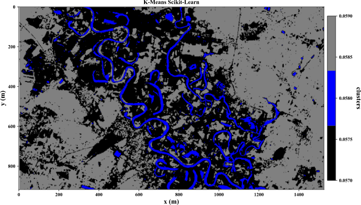
Let us crop one oxbow from the image 2D, and then extract only the waterbody.
Hint (1) use the if statement to suppress the unwanted areas. Once you extracted the waterbody successfully, you can count the number of pixels to estimate the size of the waterbody. Hint (2) use for-loop to count values in the 2D matrix that is larger and equal to your waterbody values.
oxbow

Flatten Matrix to Sequential Order (Vector)
\mathbf{A} \in \mathbb{R}^{4\times 3}
\mathbf{a_{0, 1}}
\mathbf{a_{0, 2}}
\mathbf{a_{1, 0}}
\mathbf{a_{1, 1}}
\mathbf{a_{1, 2}}
\mathbf{a_{2, 0}}
\mathbf{a_{2, 1}}
\mathbf{a_{2, 2}}
\mathbf{a_{3, 0}}
\mathbf{a_{3, 1}}
\mathbf{a_{3, 2}}
\mathbf{a} \in \mathbb{R}^{12}
\mathbf{a_{0, 1}}
\mathbf{a_{0, 2}}
\mathbf{a_{1, 1}}
\mathbf{a_{1, 2}}
\mathbf{a_{2, 0}}
\mathbf{a_{2, 1}}
\mathbf{a_{2, 2}}
\mathbf{a_{3, 0}}
\mathbf{a_{3, 1}}
\mathbf{a_{3, 2}}
\mathbf{a_{1, 0}}
\mathbf{a_{0, 0}}
\mathbf{a_{0, 0}}
\mathbf{a_{0, 1}}
\mathbf{a_{0, 2}}
\mathbf{a_{1, 0}}
\mathbf{a_{1, 1}}
\mathbf{a_{1, 2}}
\mathbf{a_{2, 0}}
\mathbf{a_{2, 1}}
\mathbf{a_{2, 2}}
\mathbf{a_{3, 0}}
\mathbf{a_{3, 1}}
\mathbf{a_{3, 2}}
\mathbf{a} \in \mathbb{R}^{12}
\mathbf{a_{0, 1}}
\mathbf{a_{0, 2}}
\mathbf{a_{1, 1}}
\mathbf{a_{1, 2}}
\mathbf{a_{2, 0}}
\mathbf{a_{2, 1}}
\mathbf{a_{2, 2}}
\mathbf{a_{3, 0}}
\mathbf{a_{3, 1}}
\mathbf{a_{3, 2}}
\mathbf{a_{1, 0}}
\mathbf{a_{0, 0}}
\mathbf{a_{0, 0}}
\mathbf{A} \in \mathbb{R}^{4\times 3}
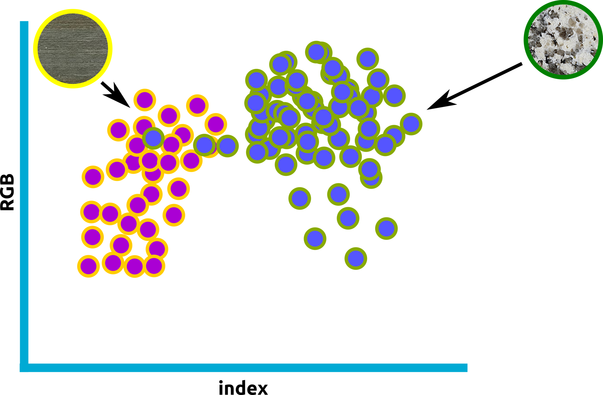
One of the most common technique in ML that has many applications such as speed up the ccomputation, sinking high-dimentional space into vector for compuation.
Show me how you flatten the 2D array
import numpy as np

x = np.array([1, 2, 3, 4, 12, 4.6, -2])
y = np.array([5, 8, 9, -1, -8.3, 2.6, 0])

dummy_of_2D = np.zeros(shape=(len(y), len(x)), dtype=float)
for col in range (0, len(x)):
    print('second loop x =', x[col])
    for row in range (0, len(y)):
        # print('first loop x =', x[col], 'first loop y =', y[row])
        dummy_of_2D[row, col] =+ x[col] + y[row]
print(dummy_of_2D.shape)
print(dummy_of_2D)
Flatten Matrix to Sequential Order (Vector)
Revisit Latent Space
255
208
2
255
127
255
106
255
8
255
vector
Game for Weekend
x < 4.2
A > 80
A > 80
0
2
4
6
8
2
4
6
8
10
CH 2: INTRODUCTORY
MACHINE LEARNING
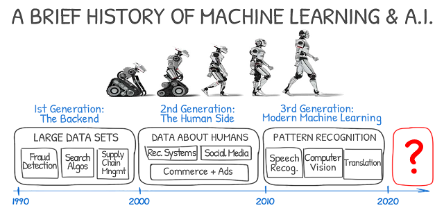
ML Timeline

Extracting Subsurface Information Using Well Logs
Data Types: Tabular (Well Logs)
| Facies | Formation | Well Name | Depth | GR | ILD_log10 | DeltaPHI | PHIND | PE | NM_M | RELPOS |
|---|---|---|---|---|---|---|---|---|---|---|
| 3 | A1 SH | SHRIMPLIN | 2793 | 77.45 | 0.664 | 9.9 | 11.915 | 4.6 | 1 | 1 |
| 3 | A1 SH | SHRIMPLIN | 2793.5 | 78.26 | 0.661 | 14.2 | 12.565 | 4.1 | 1 | 0.979 |
| 3 | A1 SH | SHRIMPLIN | 2794 | 79.05 | 0.658 | 14.8 | 13.05 | 3.6 | 1 | 0.957 |
| 3 | A1 SH | SHRIMPLIN | 2794.5 | 86.1 | 0.655 | 13.9 | 13.115 | 3.5 | 1 | 0.936 |
| 3 | A1 SH | SHRIMPLIN | 2795 | 74.58 | 0.647 | 13.5 | 13.3 | 3.4 | 1 | 0.915 |
| 3 | A1 SH | SHRIMPLIN | 2795.5 | 73.97 | 0.636 | 14 | 13.385 | 3.6 | 1 | 0.894 |
| 3 | A1 SH | SHRIMPLIN | 2796 | 73.72 | 0.63 | 15.6 | 13.93 | 3.7 | 1 | 0.872 |
| 3 | A1 SH | SHRIMPLIN | 2796.5 | 75.65 | 0.625 | 16.5 | 13.92 | 3.5 | 1 | 0.83 |
| 3 | A1 SH | SHRIMPLIN | 2797 | 73.79 | 0.624 | 16.2 | 13.98 | 3.4 | 1 | 0.809 |
numberic data
integer
floating-point
categorical data
binary
muticlass
text
string
Facies: 3, NM_M: 1
Depth: 2793.0, GR: 78.26
Facies: 2 classes
Facies: 9 classes
data
types
Well Name: SHRIMPLIN
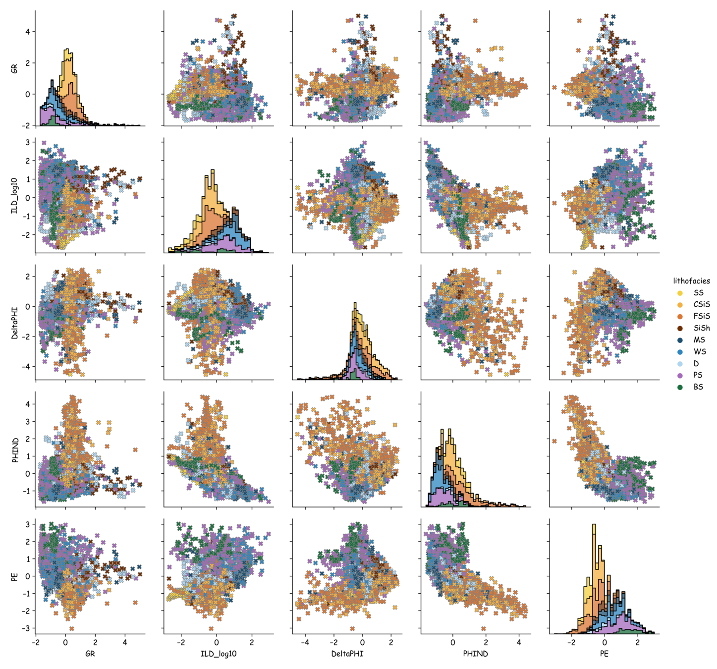
Data Correlation (Scatter Plot)

Tabular data provide a lot of information contained multiple rows and columns, and these big data might need to decompose into a scatter plot to gain more understanding about the data. Here, we analyze the relationship between ILD and GR. Note that one log penetrates through multi-layers of rocks showing on the left diagram as multiple colors.
Let us try to reproduce the figure. Note that if you would like to sampling data such as every 10 data points and show only one point, you can use "data = data[::10]".

Data Correlation (Linear Regression)

input data
create line to fit
measuring the error
find the best fit


\Delta x
\Delta y
slope = \Delta x / \Delta y
intercept = line\ cross\ axis-y
Unsupervised Learning (K-means)
input data
locate centroids
measure distances
relocate centroids
distance equal threshold
end
yes
no


find the shortest paths between each data point and centroid.
yes/no condition, the program will end if the shortest distances between centroids and data points equal the threshold (near 0)

done! good job
Demo K-Means


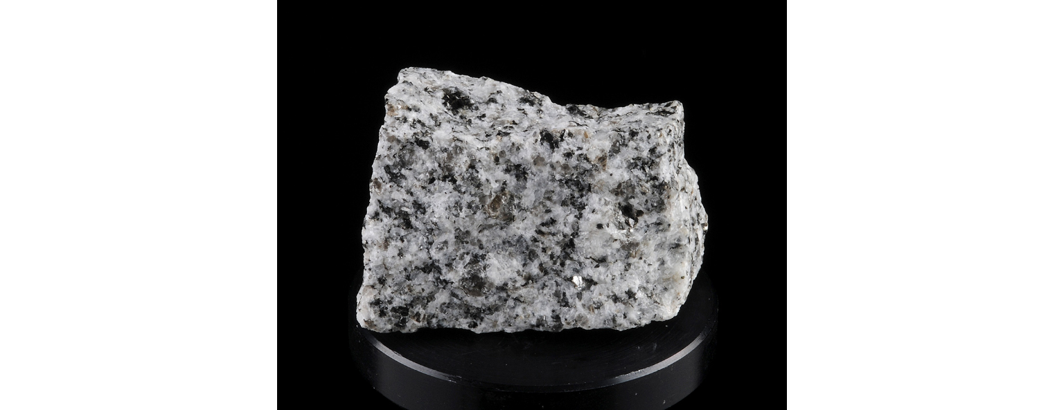
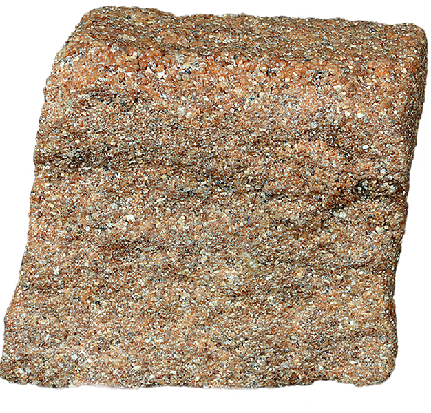
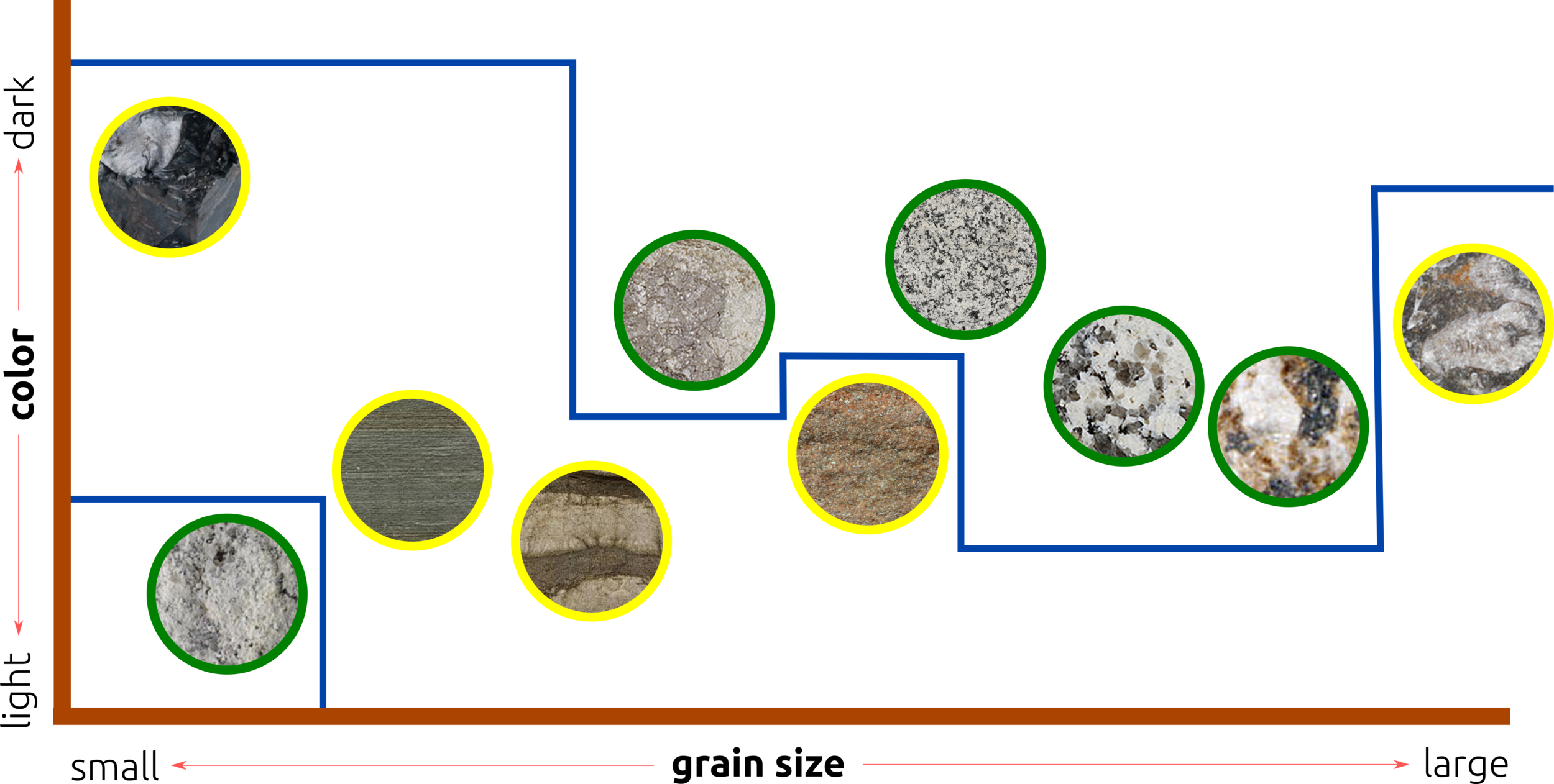
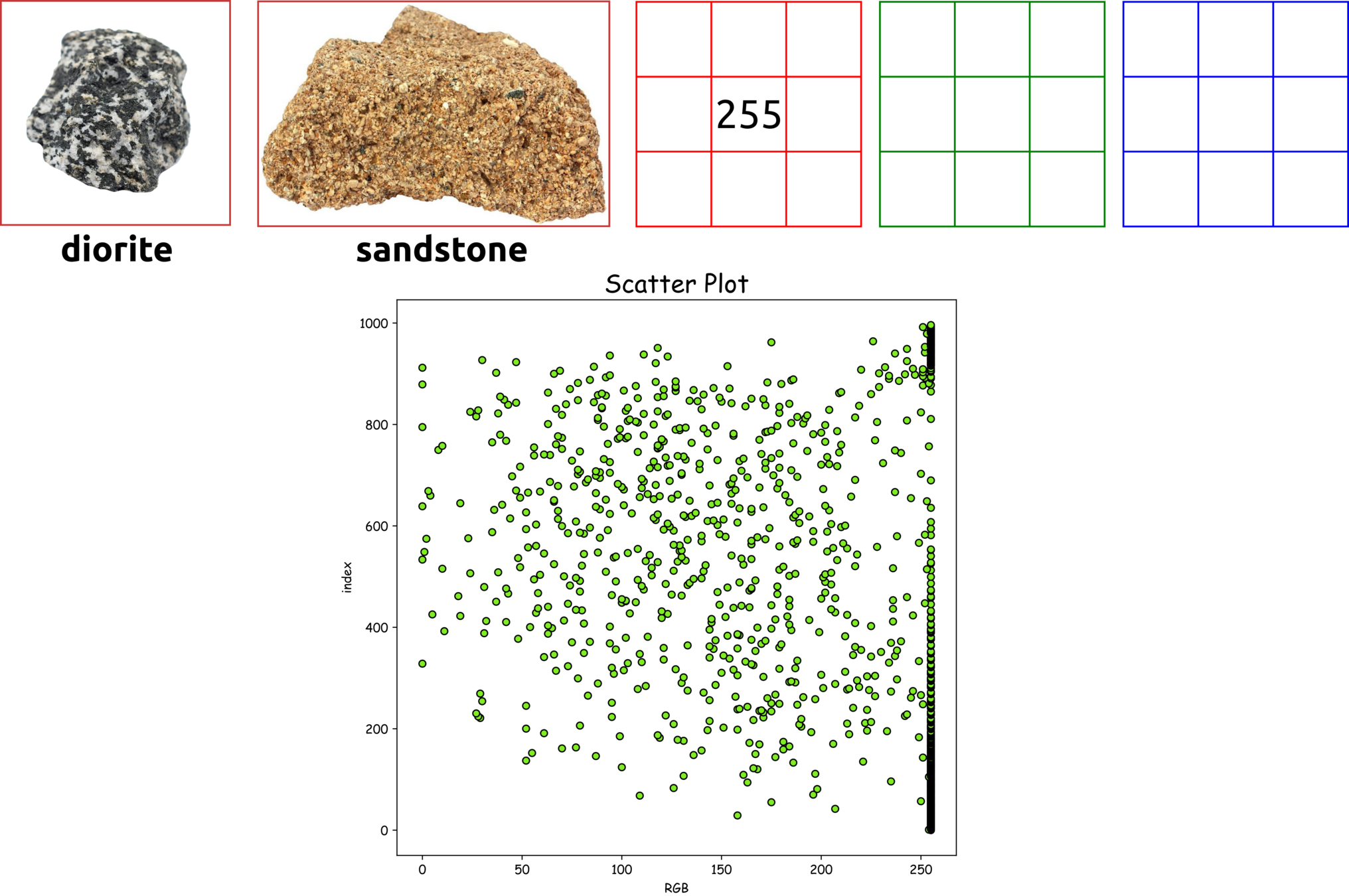
Supervised Learning (Decision Tree)
classify granite and sandstone
grain size
<0.1
>=0.1
color
white-like
dark-like
density
mineral
>=2.60
hardness
<2.60
Mohs = 1
Mohs = 7
Mohs = 10
quartz
felspar
granite
sandstone
keep in mind that we can not classify granite and sandstone such as these simple rules.

balanced decision trees


1
2
4
3
Decision Tree (Example)
preview a result from this exercise

CH 3: PREPROCESSING DATA
Normalization

normalization

Outliers

outlier

Demo Normalization and Outliers


drop outlier

Preprocessing Data
missing values
normalization
outliers
categorical transformation
| Facies | Formation | Well Name | Depth | GR | ILD_log10 | DeltaPHI | PHIND | PE | NM_M | RELPOS |
|---|---|---|---|---|---|---|---|---|---|---|
| sand | A1 SH | SHRIMPLIN | 2793 | 77.45 | 0.664 | 9.9 | 11.915 | 4.6 | 1 | 1 |
| shale | A1 SH | SHRIMPLIN | 2793.5 | 78.26 | 0.661 | 14.2 | 12.565 | 4.1 | 1 | 0.979 |
| dolomite | A1 SH | SHRIMPLIN | 2794 | 79.05 | 0.658 | 14.8 | 13.05 | 3.6 | 1 | 0.957 |
| sand | A1 SH | SHRIMPLIN | 2794.5 | 86.1 | 0.655 | 13.9 | 100 | 3.5 | 1 | 0.936 |
| shale | A1 SH | SHRIMPLIN | 2795 | 74.58 | 0.647 | 13.3 | 3.4 | 1 | 0.915 | |
| limestone | A1 SH | SHRIMPLIN | 2795.5 | 73.97 | 0.636 | 14 | 13.385 | 3.6 | 1 | 0.894 |
| dolomite | A1 SH | SHRIMPLIN | 2796 | 73.72 | 0.63 | 15.6 | 13.93 | 3.7 | 1 | 0.872 |
| sand | A1 SH | SHRIMPLIN | 2796.5 | 75.65 | 0.625 | 16.5 | 13.92 | 3.5 | 1 | 0.83 |
| sand | A1 SH | SHRIMPLIN | 2797 | 73.79 | 0.624 | 16.2 | 13.98 | 3.4 | 1 | 0.809 |
-999
(13.9+14)/2
| Facies | categorical transformation |
|---|---|
| sand | 1 |
| shale | 2 |
| dolomite | 3 |
| sand | 1 |
| shale | 2 |
| limestone | 4 |
| dolomite | 3 |
| sand | 1 |
| sand | 1 |
min
max
-1
1
73.72
0.624
86.1
0.664
75.65
0.647
???
Demo Missing Value in Decision Tree
import data
step 1
preprocessing data
step 2
split data
step 3
decision tree
evaluate model
step 4
step 5

| PE | miss_value |
|---|---|
| 4.6 | 0 |
| 4.1 | 0 |
| 3.6 | 0 |
| -999 | 1 |
| -999 | 1 |
| -999 | 1 |
| -999 | 1 |
| -999 | 1 |
| -999 | 1 |

try to compare between add one more column of missing value and without adding the column
try to compare between add one more column of missing value and without adding the column
This time change ratio of splitting data and max depth
Note that this demo preprocessing only missing values by adding one column. Future work can apply dropping outliers, normalization, etc.
1. Binomial classification: predicting two-class (e.g., yes or no)
2. Multinomial classification: predicting more than two-class
3. Hybrid to binary: force predicting of more classes into two classes
3.1 one vs the rest
3.2 one? vs one?
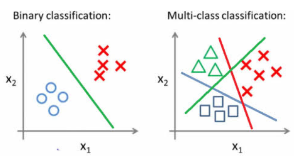
3 Types of Classification Methods in AutoML
Demo Missing Value in Decision Tree

import data
step 1
preprocessing data
step 2
split data
step 3
decision tree
evaluate model
step 4
step 5
step 4
CH 4: AUTOMATIC
MACHINE LEARNING
How Does AutoML Improve Pipeline in ML/DL?
input data
feature engineering
inference
evaluation metrics
ML Model(s)
inference
SVM
GTB
K-means
AutoML
lightGBM
RF
neuron network
XGBoost
CatBoost
algorithm selection with optimized parameters
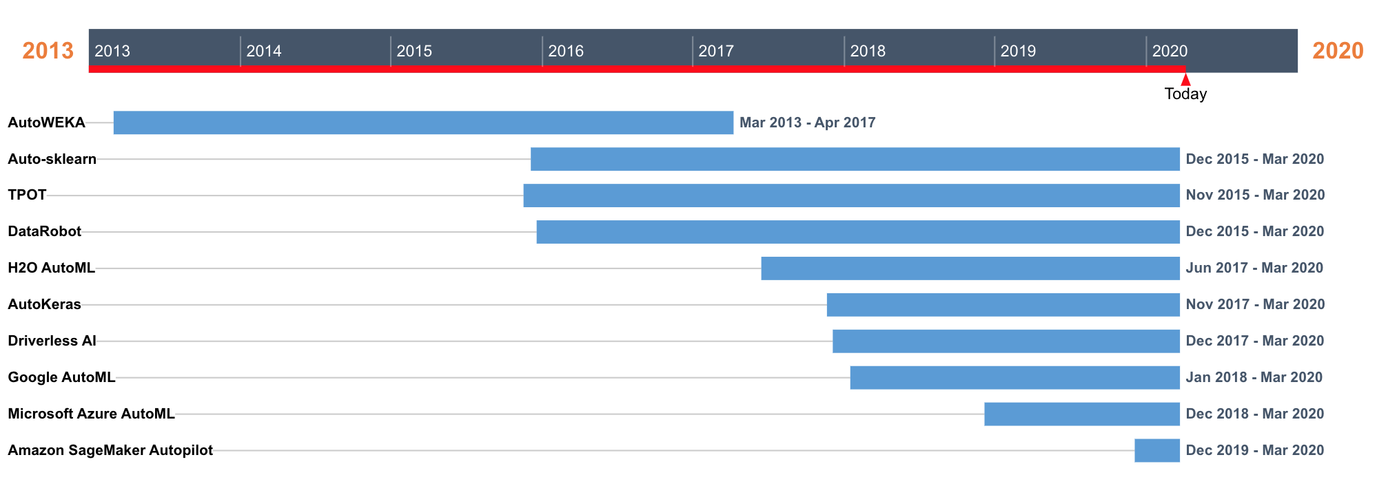
The Past, Present, Future of AutoML

A Demo Project on Well Log Analysis
The figures show that the intervals contain sequence stratigraphy of fluvial environment exposed to the surface. Geoscientists can interpret the rocks based on colors, gain sizes, and minerals. So how can we obtain the subsurface information?


In order to obtain that information, geoscientists deploy wirelines into a borehole to measure a formation property. Each rock layer contained different kinds of minerals that possess distinguishable characteristics. However, their properties are not discrete, which requires tremendous works to classify. Here, we will follow the SEG competition 2016 to study ML/AutoML workflow to create a robotized framework of petrophysical analysis.
AutoML Pipeline
input data
continued

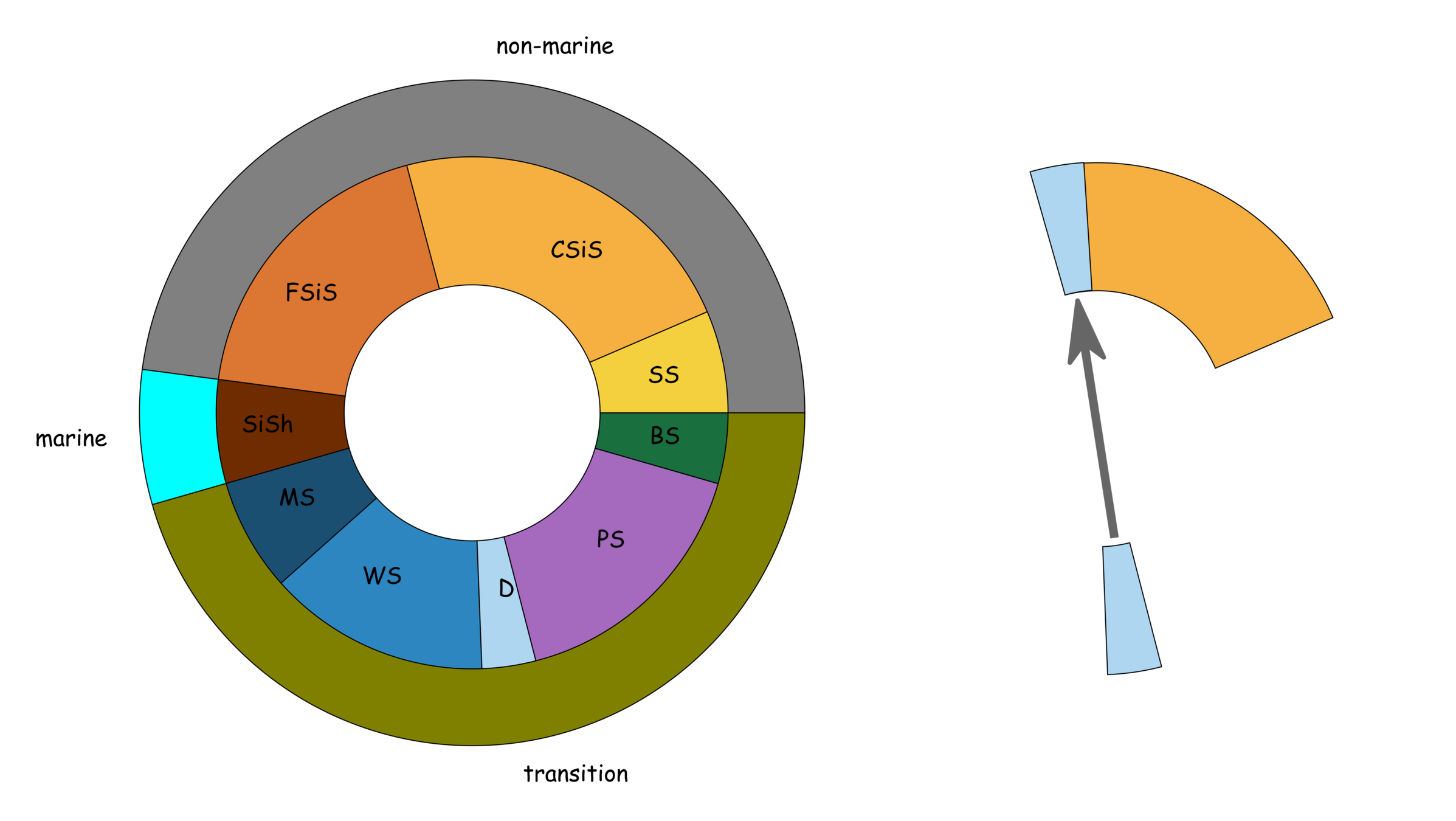
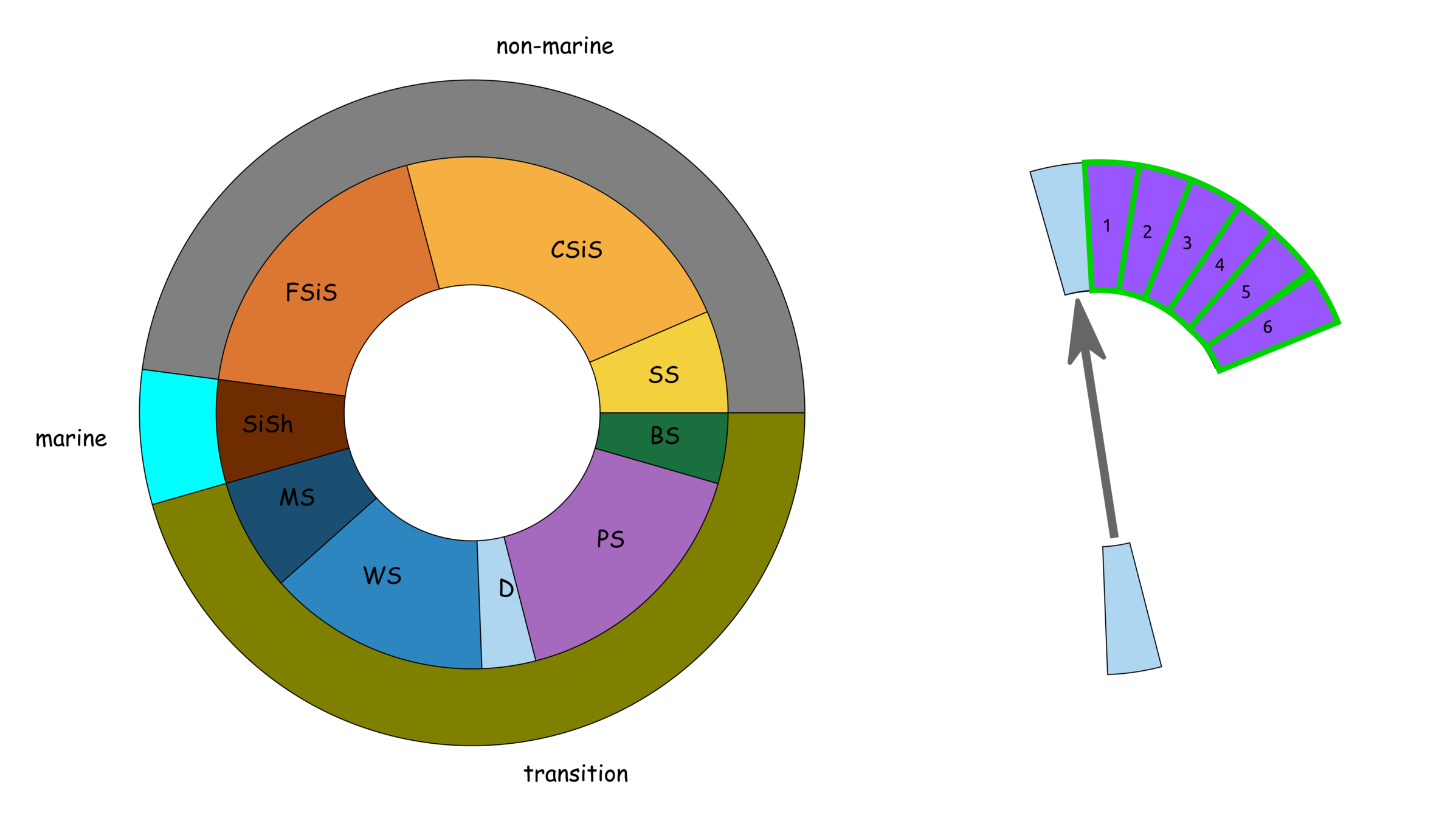
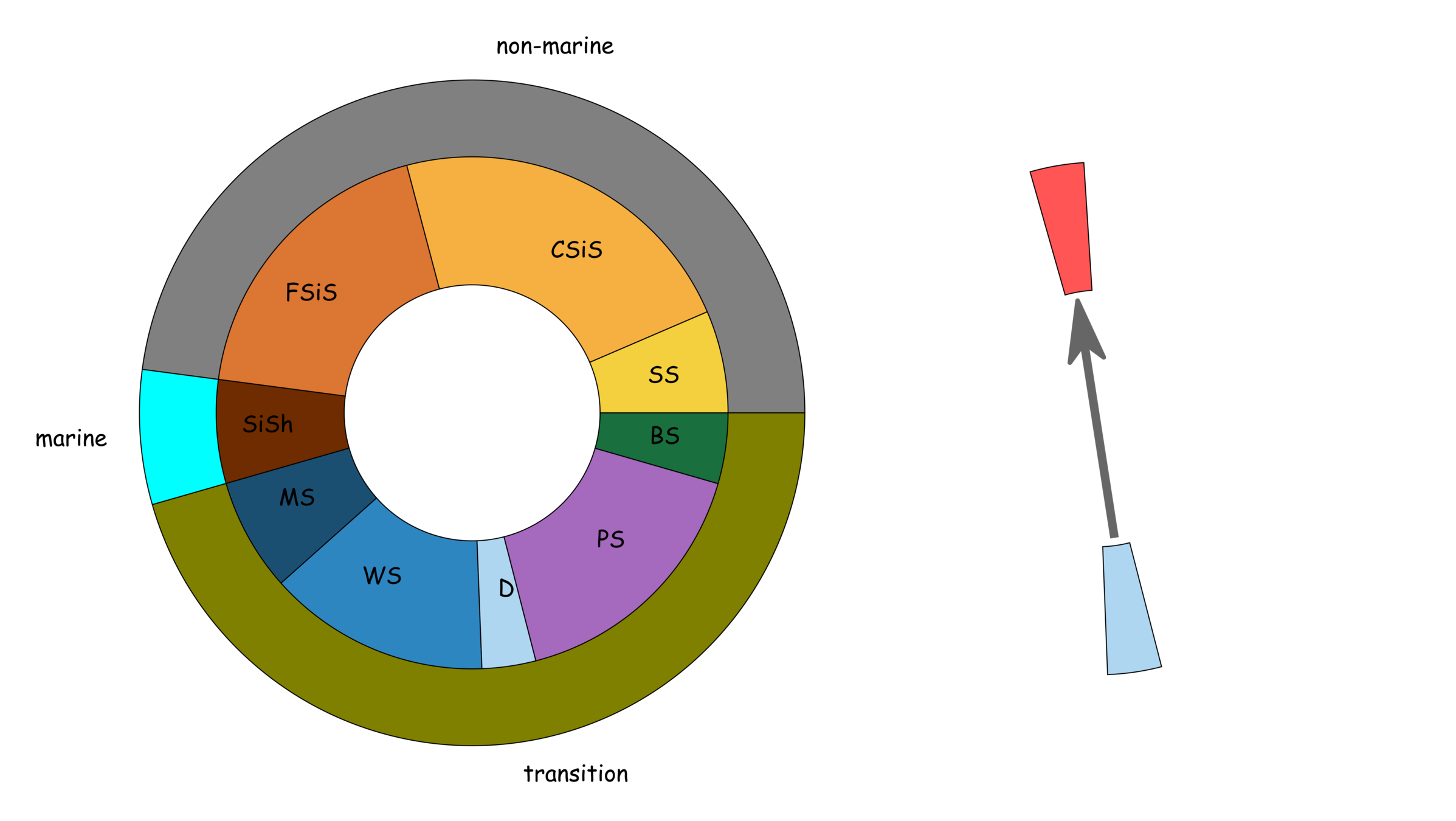
lithofacies
well log (Newby)
pairplots with normal distributions
Facies description labels with adjacent facies
|
1 |
Nonmarine sandstone |
|
2 |
|
2 |
Nonmarine course siltstone |
|
1,3 |
|
3 |
Nonmarine fine siltstone |
|
2 |
|
4 |
Marine siltstone and shale |
|
5 |
|
5 |
Mudstone |
|
4,6 |
|
6 |
Wackestone |
|
5,7,8 |
|
7 |
Dolomite |
|
6,8 |
|
8 |
Packstone-grainstone |
|
6,7,9 |
|
9 |
Phylloid-algal bafflestone |
|
7,8 |
SS
CSiS
FSiS
SiSh
MS
WS
D
PS
BS

non-marine
marine
transition
input data
continued
feature engineering

raw data

preprocessed data
input data
continued
AutoML
feature engineering
split data by wells
split data by fraction (80%)

training data
validated data
test
NEWBY
LUKE G U
CROSS H CATTLE
SHANKLE
SHRIMPLIN
Recruit F9
NOLAN
ALEXANDER D
CHURCHMAN BIBLE
KIMZEY A

split data by fraction (20%)

training data (80%)
validating data (20%)
model list (top 5)
-
CatBoost
-
XGBoost
-
LightGBM
-
RandomForest
-
NeuralNetFastAI
model ensembling with stacking/bagging
models in AutoML
input data
continued
feature engineering
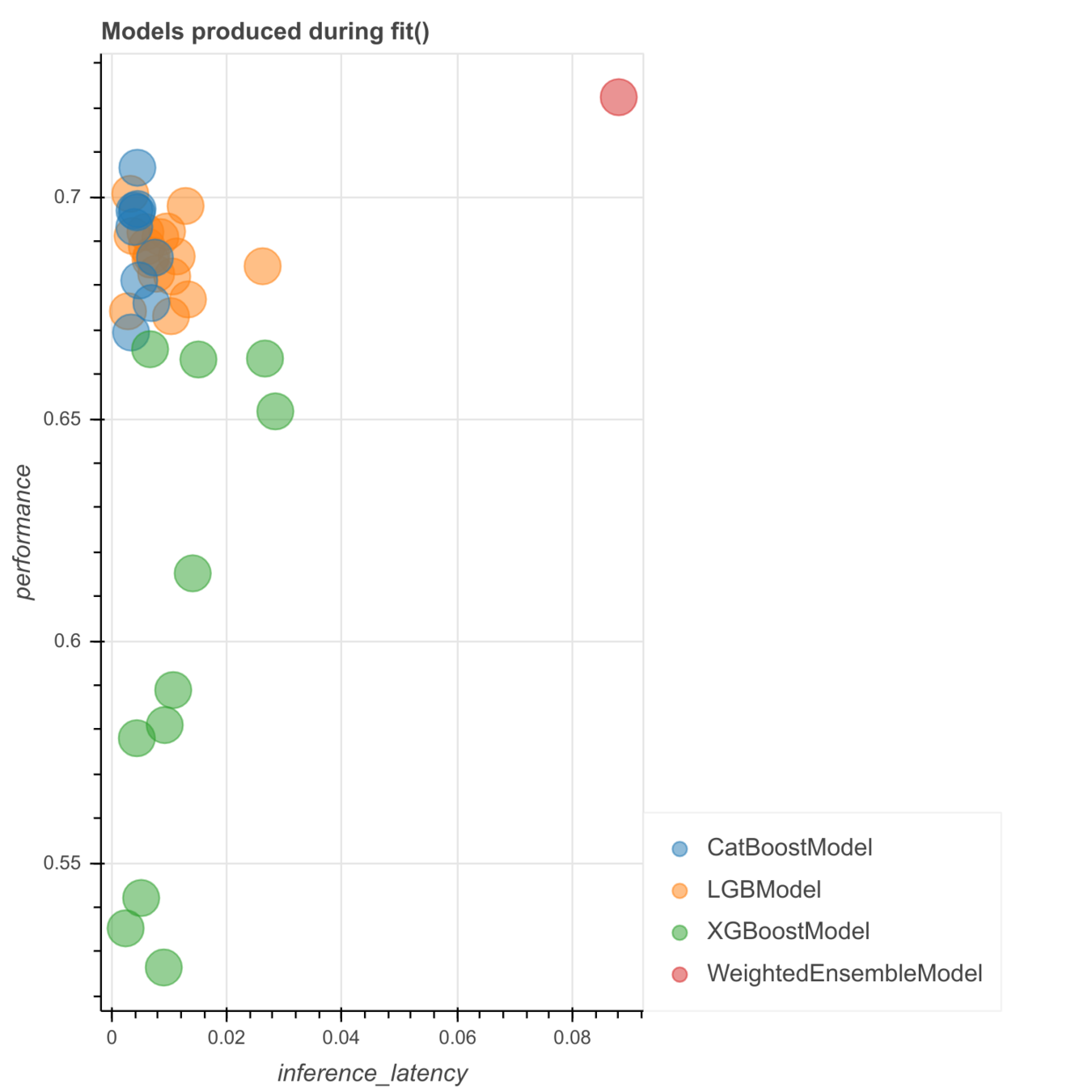
confusion matrix (WeightedEnsemble_L3)
evaluation metrics
AutoML

input data
feature engineering
AutoML
trained models
evaluation metrics
Done! GOOD JOB
Weighted_Ensemble_L3 (f1 macro: 0.311)

Facies description labels with adjacent facies
|
1 |
Nonmarine sandstone |
|
2 |
|
2 |
Nonmarine course siltstone |
|
1,3 |
|
3 |
Nonmarine fine siltstone |
|
2 |
|
4 |
Marine siltstone and shale |
|
5 |
|
5 |
Mudstone |
|
4,6 |
|
6 |
Wackestone |
|
5,7,8 |
|
7 |
Dolomite |
|
6,8 |
|
8 |
Packstone-grainstone |
|
6,7,9 |
|
9 |
Phylloid-algal bafflestone |
|
7,8 |
SS
CSiS
FSiS
SiSh
MS
WS
D
PS
BS

Confusion Matrix (Binary)
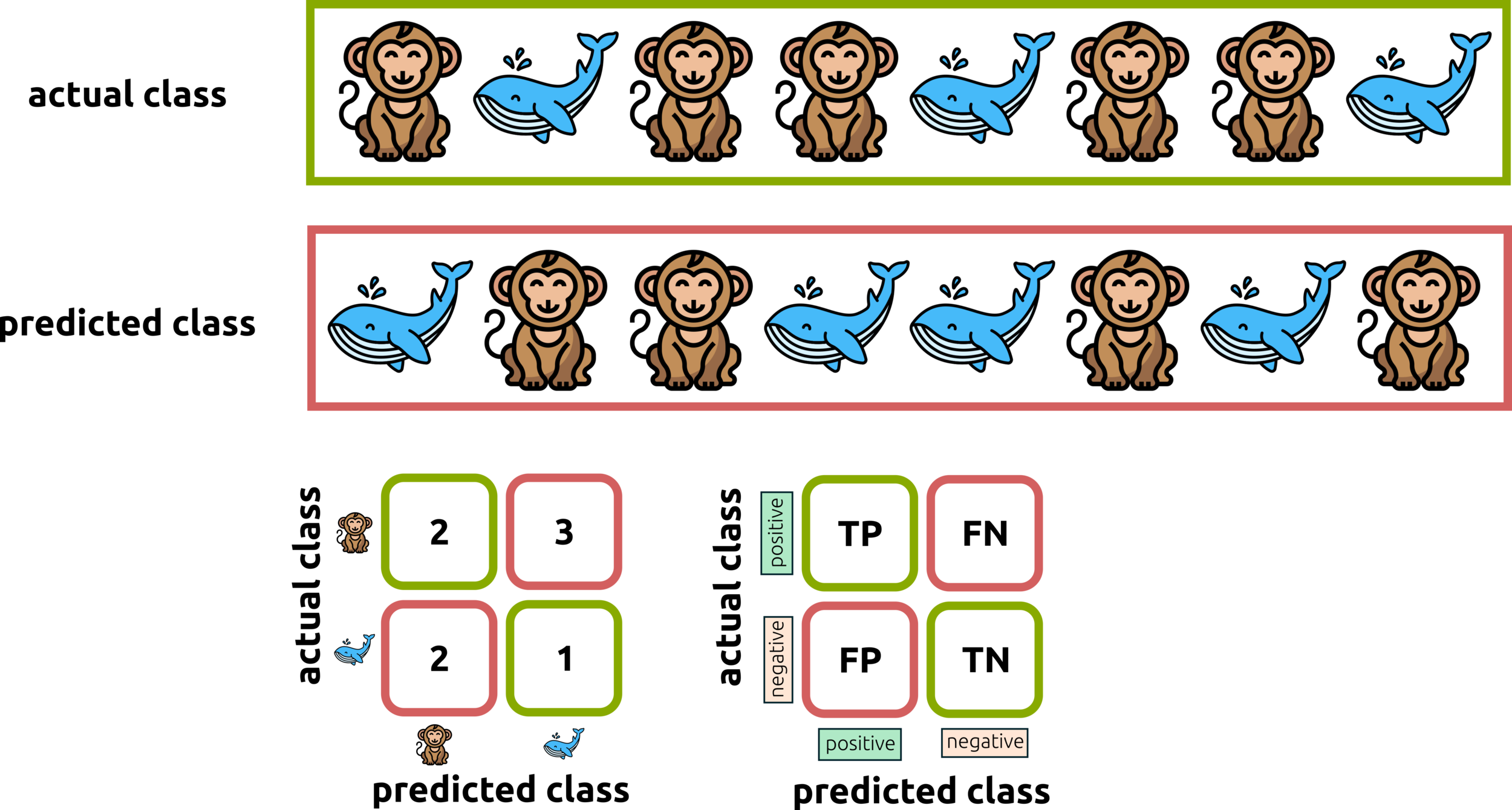
we are looking for monkey and non-monkey
Confusion Matrix (Multi-Class Classification)
prediction
TRUE POSITIVE (TP) = 10
true
hydrocarbon
brine
unsaturation
unsaturation
10
8
1
hydrocarbon
43
20
50
brine
6
70
100
unsaturation
TRUE NEGATIVE (TN) = 20+50+70+100
FALSE NEGATIVE (FN) = 43+6
FALSE POSITIVE (FP) = 8+1
Consider class-by-class (hydrocarbon)
prediction
Global and Macro Scores (All Classes vs Single Class)
\displaystyle precision=\frac{TP}{TP+FP}
\displaystyle recall=\frac{TP}{TP+FN}
\displaystyle F-1\ score=\frac{2TP}{2TP+FP+FN}
class
precision
recall
F-1 score
hydrocarbon
brine
unsaturation
CH 5: GRADIENT BOOSTED DECISION TREES (GBDTs)
Linear Regression and Gradient Descent


Linear Regression and Gradient Descent

Gradient Boosting Methods
input data
feature engineering
evaluation metrics
AutoML
trained models
gradient boosting methods
CatBoost
XGBoost
lightGBM
model ensembling with stacking/bagging
CatBoost: Gradient Boosting with
Categorical Features Support
balanced decision trees
1
2
4
3

Label-Encoding and One-Hot-Encoder
To improve the efficiency of the gradient boosting methods, we should convert all columns containing categorical data into numeric data. Label-encoding and one-hot-encoder aim to treat this problem. Label-encoding can convert categorical data into numeric data having sequential values. However, this method might implement a bias weight into a more considerable value. To overcome this problem, we use a one-hot-encoder to distribute the converted numeric column from label-encoder to have more columns, and each column contains only binary data.


Imbalanced Data

input
imbalance
oversampling
undersampling
SMOTE: Synthetic Minority Oversampling Technique
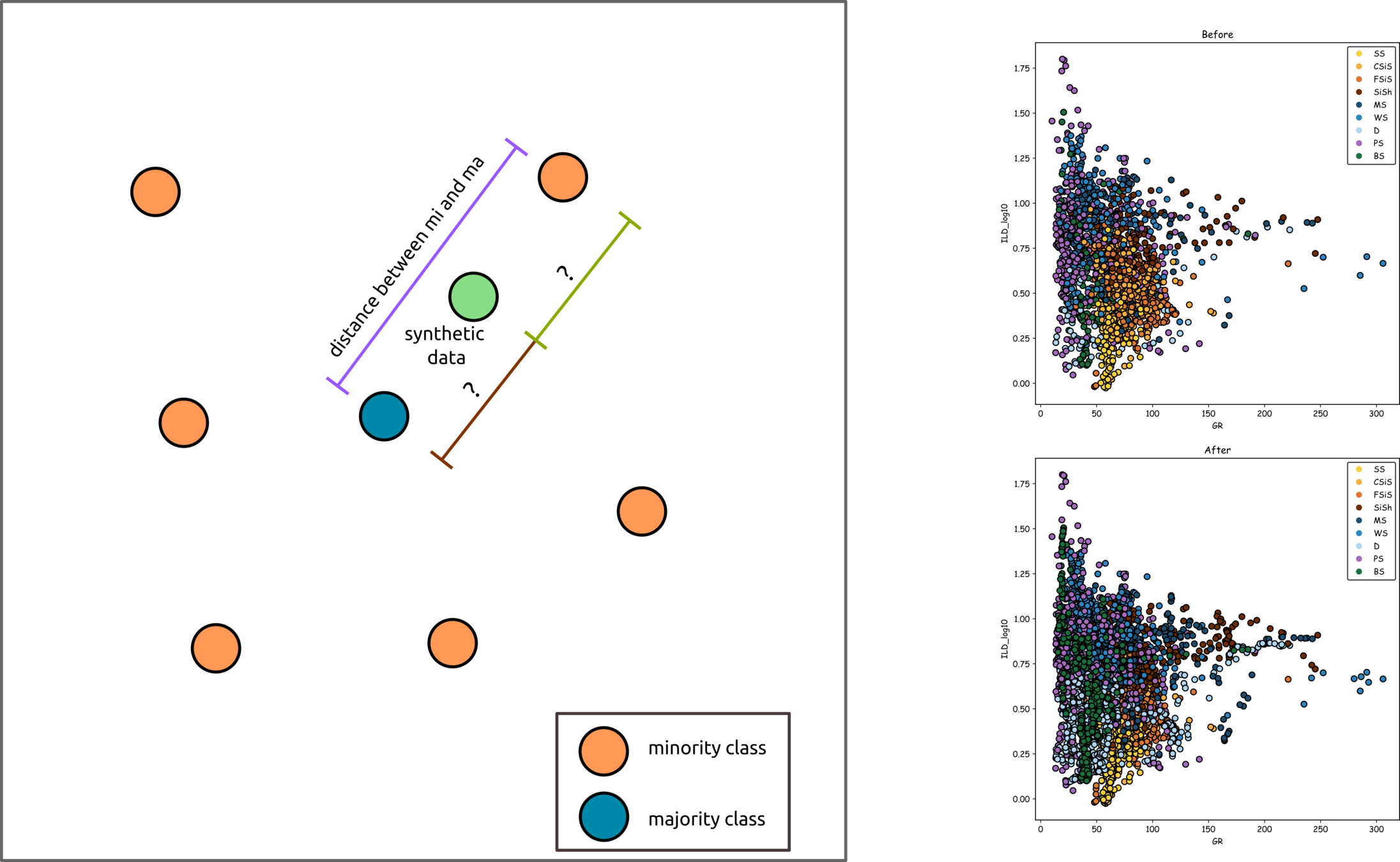
cauation
The synthetical data have one direction, which might be noise rather than data.

ADASYN: Adaptive Synthetic Sampling Approach
SMOTE + Tomek Links
SMOTE + ENN


Objectives of Cross-Validations
To answer some questions about which part of the dataset should be training and testing data, we might shuffle the data and randomly split the dataset into training and testing. Moreover, which parameters are the best for this dataset? These two questions lead data scientists to create cv techniques.

A
C
B
D
Which spilts are the best for the assigned parameters? Depend right? Practically, we should avoid depend.
Cross-Validation Types
hold-out
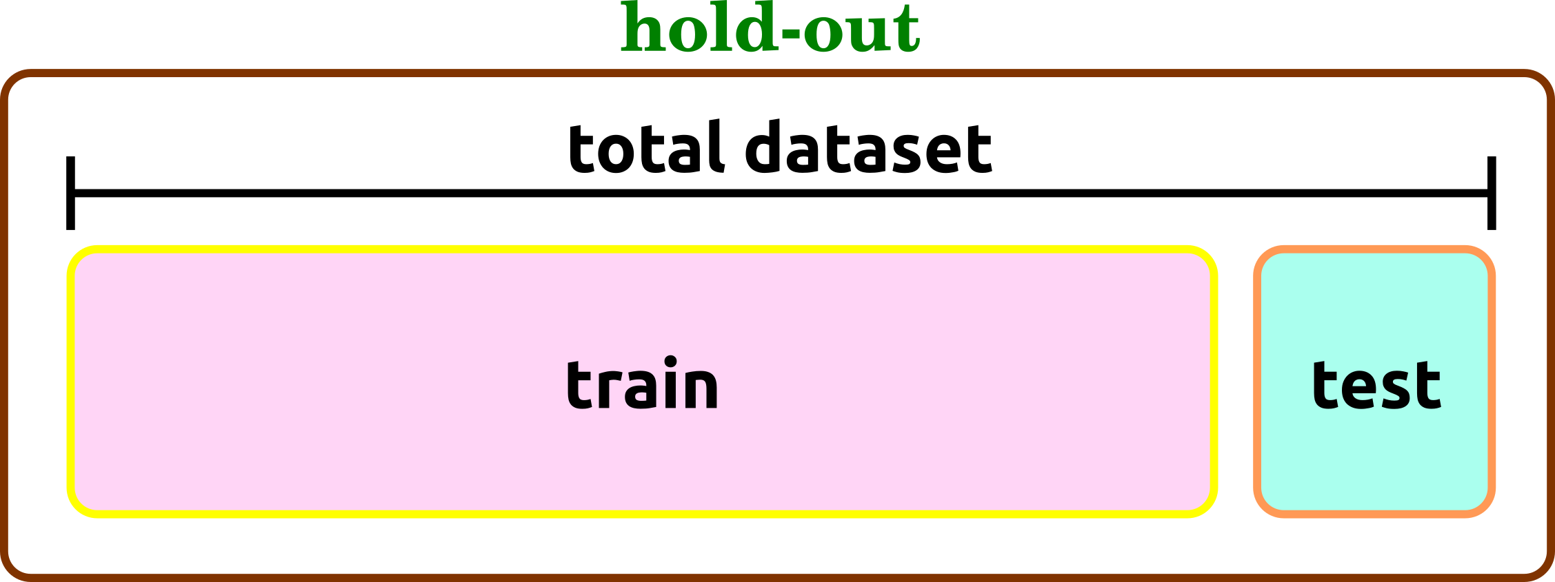
the ratio of train and test is fixed
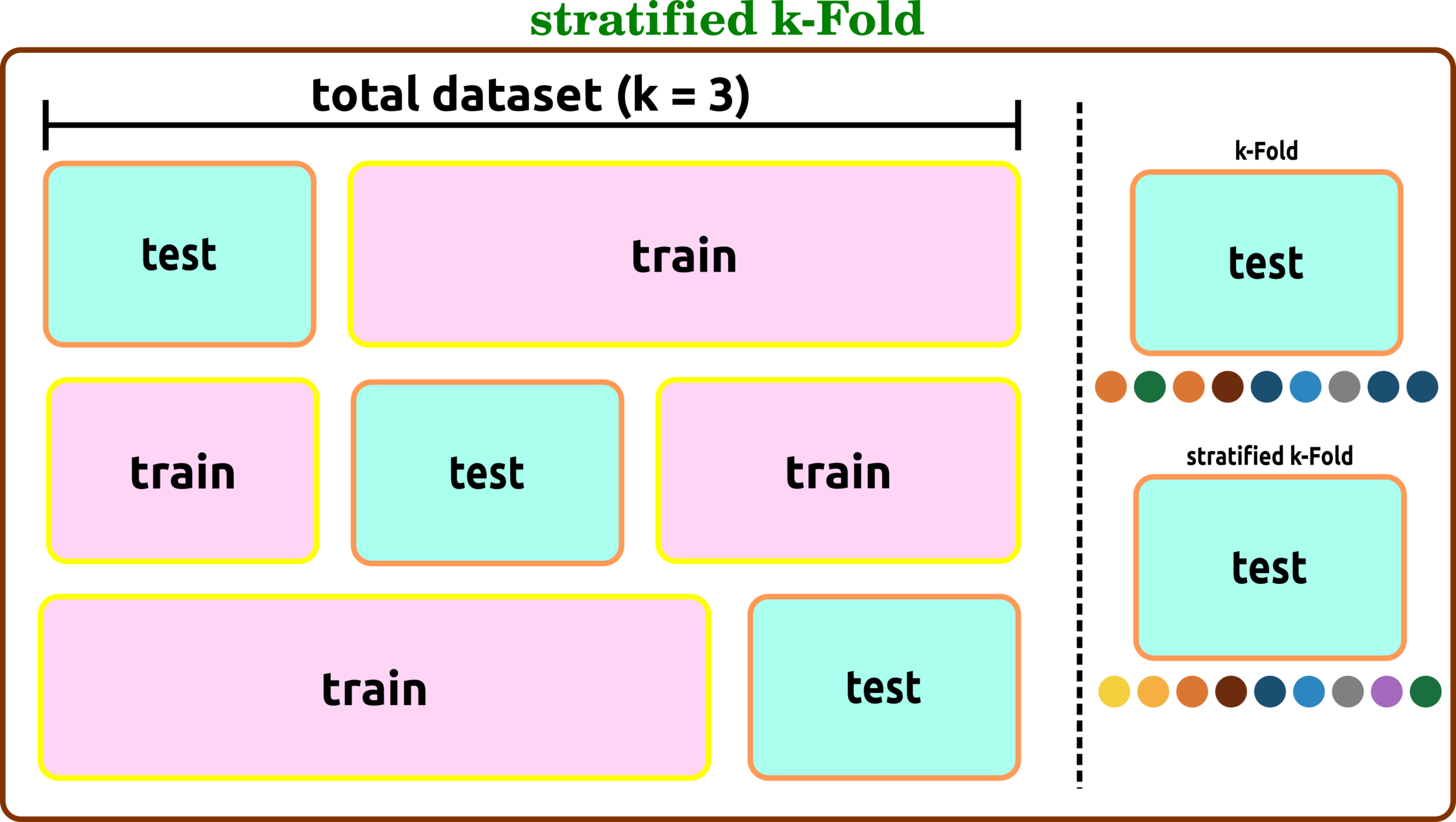
k-Fold
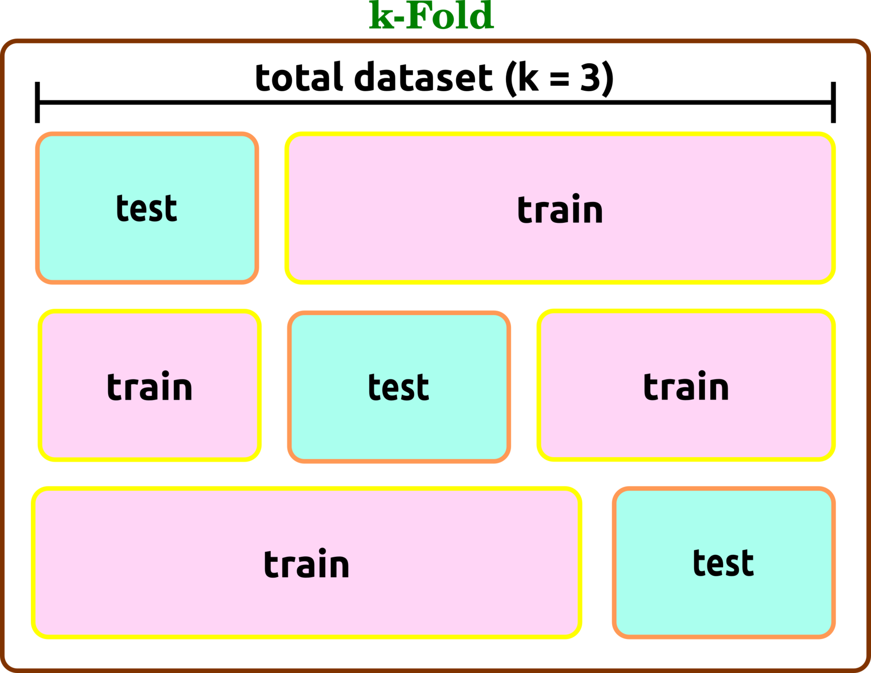
split a dataset into a number of groups (fold), so-called k, and then evaluate the model in each iteration.
repeated k-Fold
stratified k-Fold
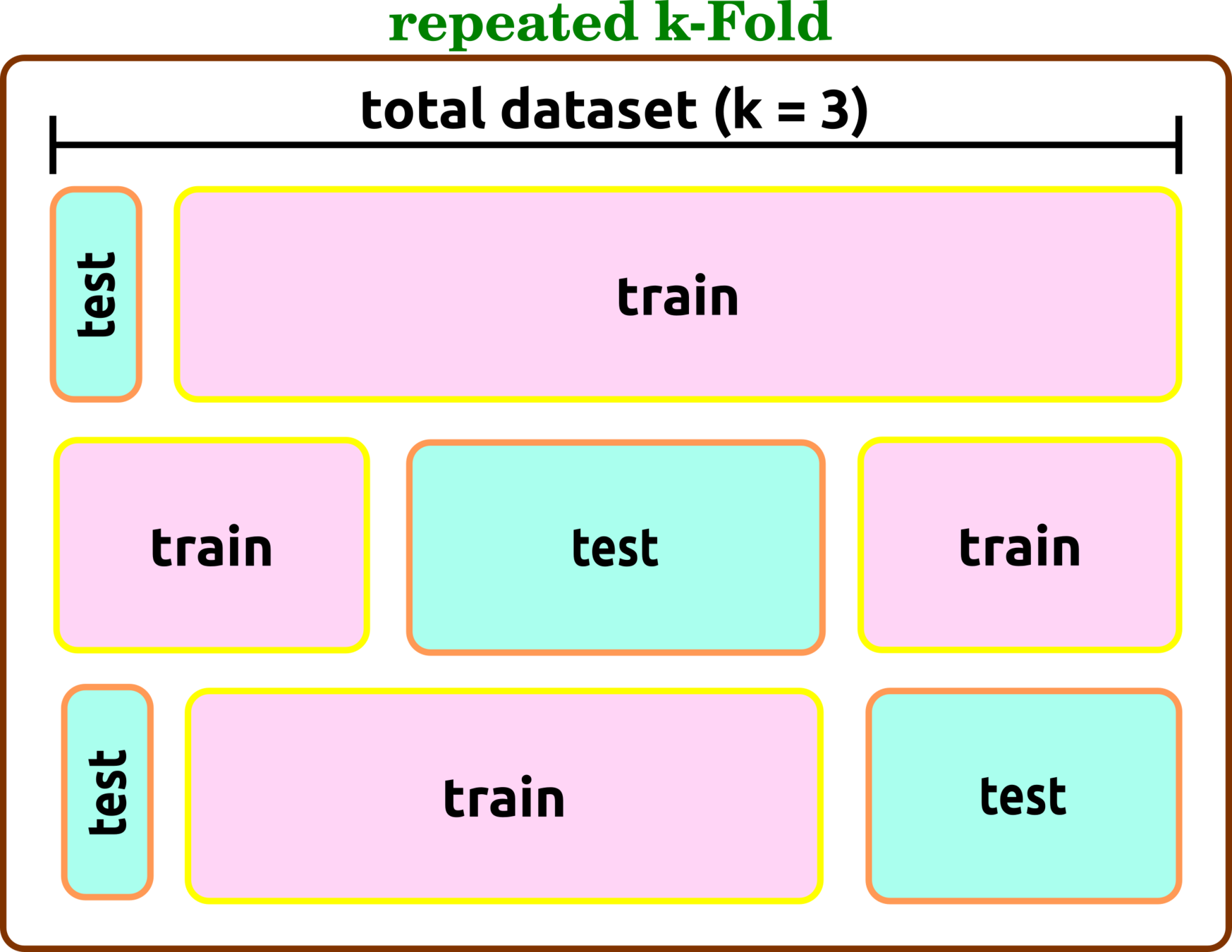
similarly with k-Fold, except the size of test data can be varied
all of the tree cv types can combine with stratified technique when test data are sorted to have all labels before evaluation.
CatBoost Multiclass Classification
input data
continued
feature engineering


normalization
outliers
missing value
encoding

input data
continued
feature engineering
CatBoost
default parameters
early stopping
over-fitting detection
model training
k-fold CV
Underfiting, Fit, and Overfitting

underfitting

fit???
overfitting

FINAL EXAM GUIDELINE
The final presentation will hold on Jan 03, 2022, starting 9.00 - 12.00. Students must turn on the camera and present for 12 mins talk, 5 mins discussion.
Submit your final presentation by Jan 02 (11.00 p.m)
Guideline
1. Compare advantages and disadvantages among pipelines. Students might design different pipelines and describe why the selected pipeline can yield the best inference.
2. Explain your code
3. Select one preprocessing that is the most important (increase/decrease f1 score or error)
4. Suppose we would like to predict only one facies, which facies should we select. Please use scientific description to address a hypothesis.
5. Suppose a new frontier area contains high shaly sand zones, from this information, which well in our dataset should use for the training model.
Questions
1. Please compare the pros and cons of applying normalization before the outlier removal.
2. List the top 2 essential parameters and show some evidence.
3. Show how to count number of facies in each well.
5. What are the limitations of using inference to predict a frontier area?
6. The method in this project is supervised or unsupervised learning?
4. Which well should not use for testing? Why?
7. Imbalanced data should apply before or after outlier removers? Why?
8. Please use educational guest, which kind of well is the most importance?
9. If we would like to bargain the exploration cost of well logs, please design your experiment to create evidence that can convince the wireline company.
10. Please design the experiment to find some hydrocarbon saturation intervals (the current dataset has no saturation information).
CH 6: HYPERPAMETER TUNING
Hyperparameter Tuning
- test all parameters
- no need for previous information
- exhausted search
- skip some parameters
- no need for previous information
- faster search
grid search
random search
parameter a
parameter b
parameter a
parameter b
Grid Search with Cross-Validation
Hyperparameter Tuning (Baysian Search)
CH 7: GAUSSIAN PROCESS REGRESSION
xxx
Copy of machine learning 2021
By pongthep


