


Content ITV PRO
This is Itvedant Content department
Business Scenario
Welcome!
Today is your 17th day as a Junior Data Analyst at a Retail Analytics Company.
The management team wants to build a Retail Sales Analysis Dashboard that provides a complete overview of business performance. The company generates thousands of transactions across different cities, categories, and sales channels. Management needs a single analytical solution that can:
Therefore, management has assigned the analytics team to build a Final Retail Sales Analysis Project that combines data analysis, visualization, and business reporting.
Git Pull
Click here to download previous lab file: DM LAB 16
git pull origin branchNameClick to download Dataset : Retail_Dataset_Cleaned
Task 1: Analyze Retail Dataset
Before creating dashboards and generating insights, analysts must ensure that the dataset is accurate, complete, and ready for analysis. Raw retail data often contains missing values, duplicate records, incorrect data types, and inconsistent values that can affect business decisions.
1
Import Required Libraries
import pandas as pd
import numpy as np
import matplotlib.pyplot as plt
import seaborn as sns
2
Load Dataset
df = pd.read_csv("/content/Retail_Dataset_Modified.csv")
print("Dataset Loaded Successfully")
Open Google Colab
3
4
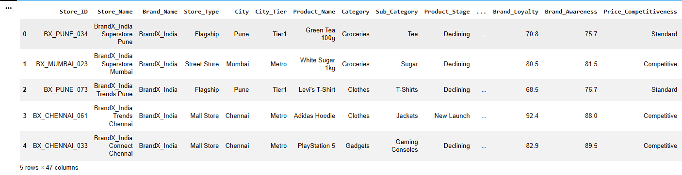
Display Dataset Information
df.head()Display First Five Records
a
b
Check Dataset Information
df.info()c
Display Statistical Summary
df.describe()5
Check Missing Values
df.isnull().sum()Convert Data Types Correctly
6
numeric_cols = [
    'Quantity_Available',
    'Units_Sold',
    'Revenue',
    'Shipping_Cost'
    ]
for col in numeric_cols:
    df[col] = pd.to_numeric(df[col], errors='coerce')
7
Handle Missing Values
Numerical Columns
a
num_cols = ['Quantity_Available', 'Units_Sold',
			'Revenue','Customer_Satisfaction',
            'Delivery_Time', 'Shipping_Cost']

for col in num_cols:
    df[col].fillna(df[col].median(), inplace=True)
b
Categorical Columns
cat_cols = ['City', 'Product_Name','Supplier']

for col in cat_cols:
    df[col].fillna(df[col].mode()[0], inplace=True)
8
Remove Duplicate Records
a
Check Duplicate Rows
df.duplicated().sum()b
Remove Duplicate Rows
df.drop_duplicates(inplace=True)c
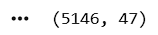
Verify Dataset Shape
df.shapeStandardize Text Formatting by Removing Extra Spaces and Correcting Capitalization
9
8
df['Category'] = df['Category'].str.strip().str.title()

df['Category'].unique()
Create New Columns
a
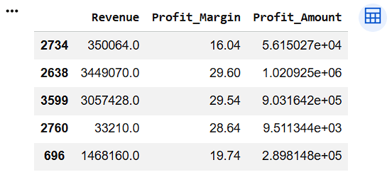
Create Profit Amount Column
df["Profit_Amount"] = (
    df["Revenue"] *
    df["Profit_Margin"] / 100
)

df[["Revenue",
    "Profit_Margin",
    "Profit_Amount"]].sample(5)
10
11
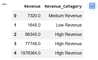
Transform Revenue into Revenue Category
df["Revenue_Category"] = np.where(
    df["Revenue"] < 5000,
    "Low Revenue",
    np.where(
        df["Revenue"] < 10000,
        "Medium Revenue",
        "High Revenue"
    )
)

df[["Revenue", "Revenue_Category"]].head()
12
8
Verify Final Dataset
df.info()df.isnull().sum()df.shapea
b
c
Task 2: Enhancing Visuals with Seaborn
Although Matplotlib creates powerful charts, building attractive statistical visualizations often requires additional customization.
Therefore, analysts use Seaborn to create visually appealing and informative charts.
What is Seaborn?
Seaborn is a Python data visualization library built on top of Matplotlib that provides beautiful statistical graphics with minimal code.
1
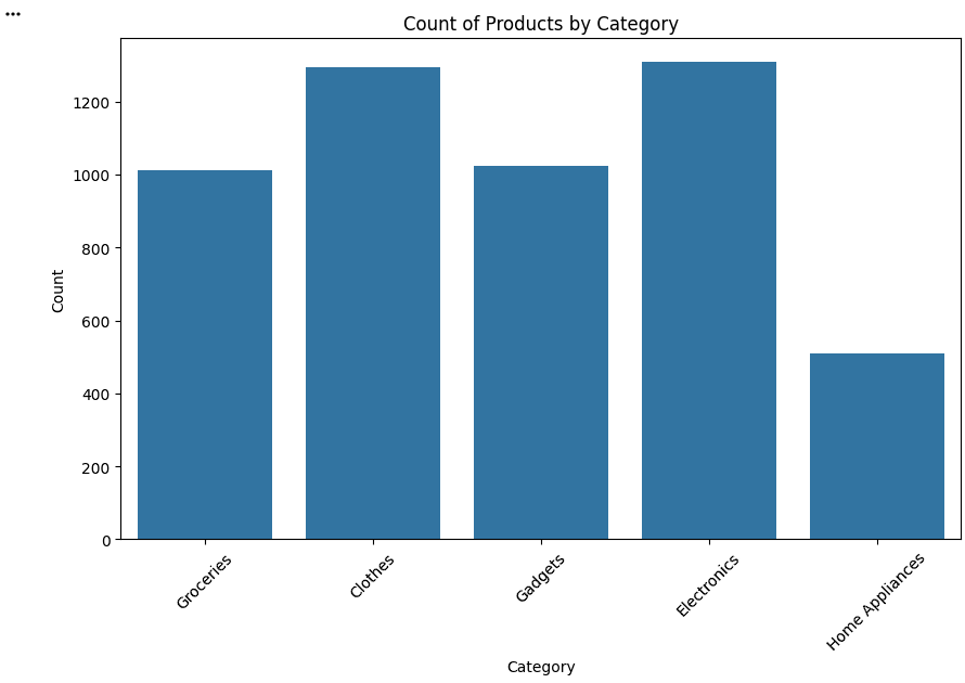
Create Category Count Plot
Display the number of records in each product category.
plt.figure(figsize=(10, 6))

sns.countplot(data=df, x='Category')

plt.title('Count of Products by Category')
plt.xlabel('Category')
plt.ylabel('Count')
plt.xticks(rotation=45)
plt.show()The countplot() function in Seaborn creates a bar chart that shows the number of occurrences (count) of each category in the Category column.
2
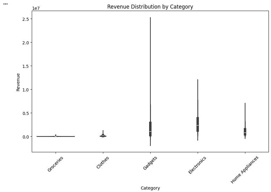
Create Revenue Violin Plot
Visualize the distribution of revenue across categories.
plt.figure(figsize=(10, 6))

sns.violinplot(data=df,
               x='Category',
               y='Revenue')

plt.title('Revenue Distribution by Category')
plt.xticks(rotation=45)

plt.show()
The violinplot() function in Seaborn creates a violin plot, which shows the distribution and density of numerical data across different categories.
3
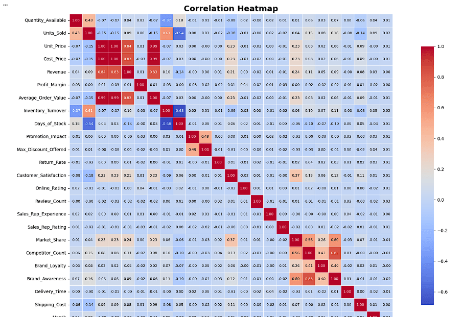
Create Correlation Heatmap
Analyze correlations among numerical variables.
# Calculate correlation matrix
corr = df.select_dtypes(include='number').corr()

# Increase figure size
plt.figure(figsize=(18, 12))
# Create heatmap
sns.heatmap(
corr,
annot=True,
fmt='.2f',
cmap='coolwarm',
linewidths=0.5,
annot_kws={'size': 8},
square=True,
cbar_kws={'shrink': 0.8}
)
# Customize chart
plt.title('Correlation Heatmap', fontsize=18, fontweight='bold')
plt.xticks(rotation=45, ha='right', fontsize=10)
plt.yticks(rotation=0, fontsize=10)
plt.tight_layout()
plt.show()corr → Correlation matrix containing relationships between numerical columns.
annot=True → Displays correlation values inside each cell.
fmt='.2f' → Shows values up to 2 decimal places.
cmap='coolwarm' → Uses blue for negative and red for positive correlations.
linewidths=0.5 → Adds borders between cells.
annot_kws={'size': 8} → Sets annotation text size to 8.
square=True → Makes each cell square-shaped.
cbar_kws={'shrink': 0.8} → Reduces the size of the color bar to 80%.
4
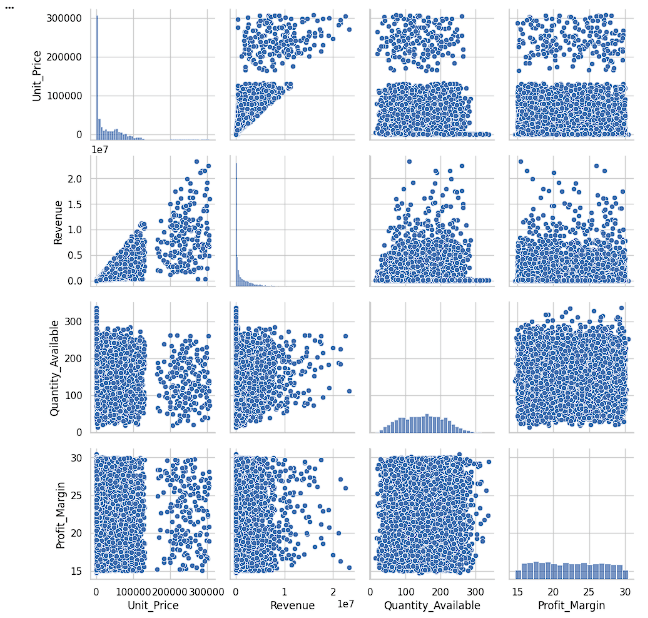
Create Pair Plot
Explore pairwise relationships among numerical features.
sns.pairplot(df[['Unit_Price',
                 'Revenue',
                 'Quantity_Available',
                 'Profit_Margin']])

plt.show()
sns.pairplot() → Creates pairwise scatter plots and distribution plots for selected numerical columns.
'Unit_Price' → Product price.
'Revenue' → Total revenue generated.
'Quantity_Available' → Available inventory quantity.
'Profit_Margin' → Profit percentage.
5
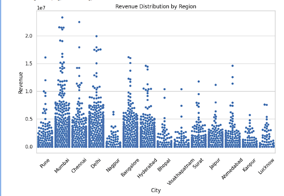
Create Revenue Swarm Plot
Visualize revenue distribution across cities.
plt.figure(figsize=(10, 6))

sns.swarmplot(data=df,
              x='City',
              y='Revenue')

plt.title('Revenue Distribution by Region')
plt.xticks(rotation=45)

plt.show()
sns.swarmplot() → Creates a scatter plot where individual data points are displayed without overlapping.
data=df → Uses the DataFrame df.
x='City' → Displays different cities on the X-axis.
y='Revenue' → Displays revenue values on the Y-axis.
6
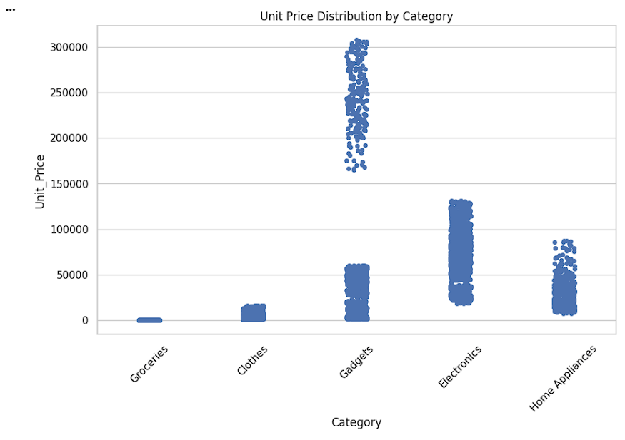
Create Unit Price Strip Plot
Display the distribution of unit prices by category.
plt.figure(figsize=(10, 6))sns.stripplot(data=df,
x='Category',
y='Unit_Price',
jitter=True)
plt.title('Unit Price Distribution by Category')
plt.xticks(rotation=45)
plt.show()sns.stripplot() → Creates a scatter plot of individual data points for categorical data.
data=df → Uses the DataFrame df.
x='Category' → Displays product categories on the X-axis.
y='Unit_Price' → Displays unit price values on the Y-axis.
jitter=True → Slightly spreads points horizontally to avoid overlapping.
7
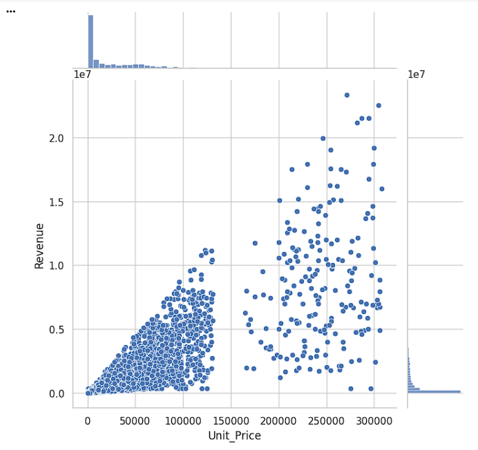
Create Joint Plot
Analyze the relationship between unit price and revenue.
sns.jointplot(data=df,
              x='Unit_Price',
              y='Revenue',
              kind='scatter',
              height=7)

plt.show()
sns.jointplot() → Creates a combined plot showing the relationship between two numerical variables and their individual distributions.
data=df → Uses the DataFrame df.
x='Unit_Price' → Displays Unit Price on the X-axis.
y='Revenue' → Displays Revenue on the Y-axis.
kind='scatter' → Creates a scatter plot to visualize the relationship.
height=7 → Sets the size of the plot to 7 inches.
8
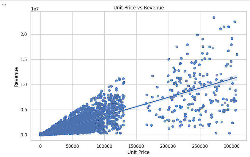
Create Regression Plot
Visualize the trend and relationship between unit price and revenue.
plt.figure(figsize=(10, 6))

sns.regplot(data=df,
            x='Unit_Price',
            y='Revenue')

plt.title('Unit Price vs Revenue')
plt.xlabel('Unit Price')
plt.ylabel('Revenue')

plt.show()
sns.regplot() → Creates a scatter plot with a fitted regression line.
data=df → Uses the DataFrame df.
x='Unit_Price' → Displays Unit Price on the X-axis.
y='Revenue' → Displays Revenue on the Y-axis.
Task 3: Customizing Charts
Business reports should be easy to understand and visually appealing.
Therefore, analysts customize charts using titles, colors, labels, and themes.
Customize Chart Appearance
1
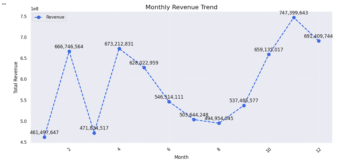
Demonstrate chart customization using titles, labels, grids, and themes.
# Apply Seaborn Theme
sns.set_theme(style="darkgrid")

# Prepare Data
monthly_revenue = df.groupby('Month')['Revenue'].sum()

# Change Figure Size
plt.figure(figsize=(12, 6))

# Create Line Chart with Color, Marker, and Line Style
plt.plot(monthly_revenue.index,
         monthly_revenue.values,
         color='royalblue',
         marker='o',
         linestyle='--',
         linewidth=2,
         markersize=8,
         label='Revenue')

# Add Title
plt.title('Monthly Revenue Trend', fontsize=16)

# Add X-axis and Y-axis Labels
plt.xlabel('Month', fontsize=12)
plt.ylabel('Total Revenue', fontsize=12)
# Rotate Axis Labels
plt.xticks(rotation=45)

# Add Grid Lines
plt.grid(True, linestyle=':', alpha=0.7)

# Add Legend
plt.legend()

# Add Annotations/Data Labels
for x, y in zip(monthly_revenue.index,
                monthly_revenue.values):
    plt.annotate(f'{y:,.0f}',
                 (x, y),
                 textcoords='offset points',
                 xytext=(0, 8),
                 ha='center')

# Adjust Layout
plt.tight_layout()

# Display Chart
plt.show()
sns.set_theme(style="darkgrid") → Applies a dark grid theme to the chart.
groupby('Month')['Revenue'].sum() → Calculates total revenue for each month.
plt.figure(figsize=(12,6)) → Sets the chart size.
plt.plot() → Creates a customized line chart.
color='royalblue' → Sets the line color to blue.
marker='o' → Adds circular markers.
linestyle='--' → Uses a dashed line.
linewidth=2 → Sets the line thickness.
markersize=8 → Sets the marker size.
label='Revenue' → Adds a label for the legend.
plt.title() → Adds the chart title.
plt.xlabel() and plt.ylabel() → Adds axis labels.
plt.xticks(rotation=45) → Rotates month labels by 45°.
plt.grid() → Adds grid lines.
plt.legend() → Displays the legend.
plt.annotate() → Displays revenue values above each point.
plt.tight_layout() → Adjusts spacing to avoid overlap.
plt.show() → Displays the final chart.
Great job!
You have successfully completed your lab on Visualize Data Using Matplotlib and Seaborn.
In this lab, you have:Created charts using Matplotlib, Built statistical visualizations using Seaborn, Customized charts with titles, labels, themes, and colors, Visualized revenue, profit, and customer satisfaction patterns, Generated business insights using retail data visualizations
You are now ready to move to the next stage of Junior Data Analyst.
Checkpoint
Git Push
git push origin branchNameBy Content ITV


