Intertemporal Choice
Christopher Makler
Stanford University Department of Economics
Econ 50: Lecture 19
Next two lectures: financial economics
Time
Risk
How much are we willing to give up now to have more later?
How much are we willing to pay to mitigate risks?
(today)
(Wednesday)
Approach: Use Tools of Consumer Theory
- Assume there is some "value function" for consumption \(v(c)\)
- Sort of like an indirect utility function
- Create "utility functions" out of this value function
- Instead of starting with some amount of money \(m\) which determines the budget line, we're going to start out with a bundle
- The "story" will describe how we can trade away from that bundle
Budget Constraint
Preferences
Utility Maximization
Cost Minimization
\text{Objective function: } u(x_1,x_2) = x_1x_2
\text{Objective function: } c(x_1,x_2) = p_1x_1 + p_2x_2
Solution functions:
"Ordinary" Demand functions
x_1^*(p_1,p_2,m) = {m \over 2p_1}
x_2^*(p_1,p_2,m) = {m \over 2p_2}
Solution functions:
"Compensated" Demand functions
x_1^c(p_1,p_2,U) = \sqrt{p_2U \over p_1}
x_2^c(p_1,p_2,U) = \sqrt{p_1U \over p_2}
What is the optimized value of the objective function?
V(p_1,p_2,m)=u(x_1^*(p_1,p_2,m),x_2^*(p_1,p_2,m))
E(p_1,p_2,U)=c(x_1^c(p_1,p_2,U),x_2^c(p_1,p_2,U))
INDIRECT UTILITY FUNCTION
EXPENDITURE FUNCTION
Utility from utility-maximizing choice,
given prices and income
Cost of cost-minimizing choice,
given prices and a target utility
Functional forms for utility / value functions:
u(x_1,x_2) = av(x_1) + bv(x_2)
v(x) = \ln x
v(x) = \sqrt{x}
v(x) = x
v(x) = x^2
u(x_1,x_2) = a \ln x_1 + b \ln x_2
u(x_1,x_2) = a \sqrt{x_1} + b\sqrt{x_2}
u(x_1,x_2) = ax_1 + bx_2
u(x_1,x_2) = ax_1^2 + bx_2^2
Cobb-Douglas (decreasing MRS)
Weak Substitutes (decreasing MRS)
Perfect Substitutes (constant MRS)
Concave (increasing MRS)
Today's Agenda
- Modeling present-future tradeoffs
- The intertemporal budget constraint
- Preferences over time
- Optimal saving and borrowing
- Different interest rates for borrowing and saving
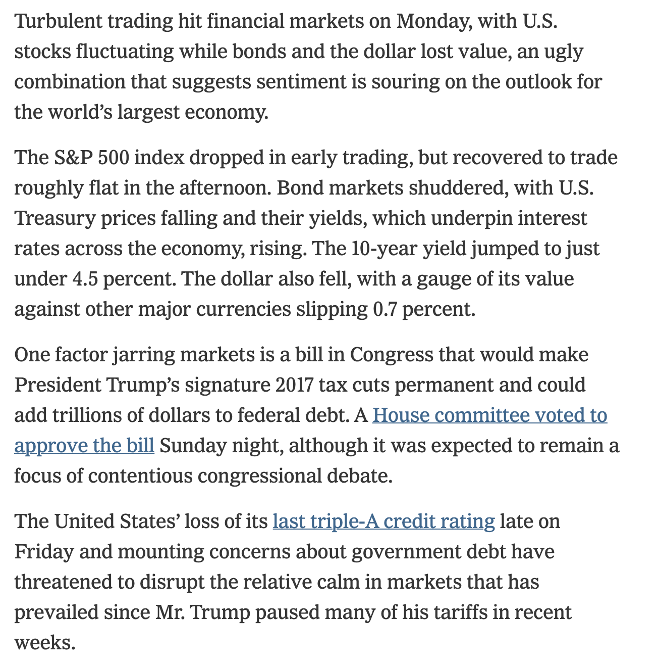
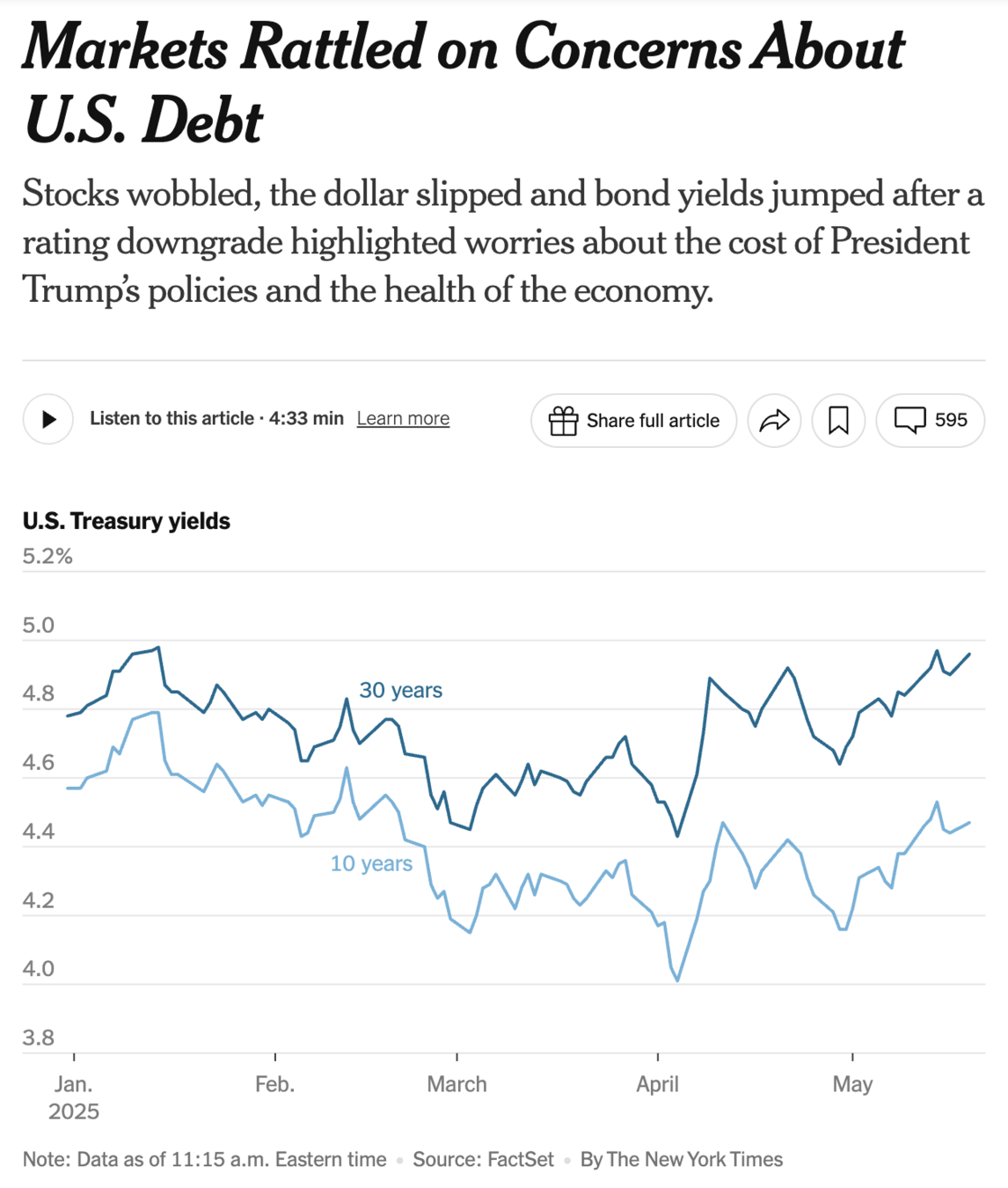
Saving and borrowing is a huge part of the U.S. economy.

Budget Line
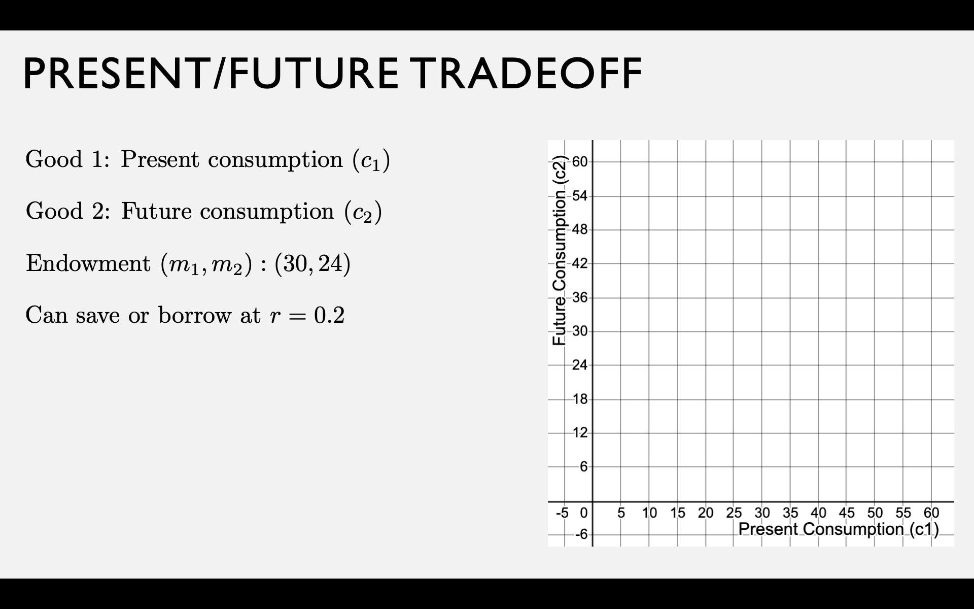
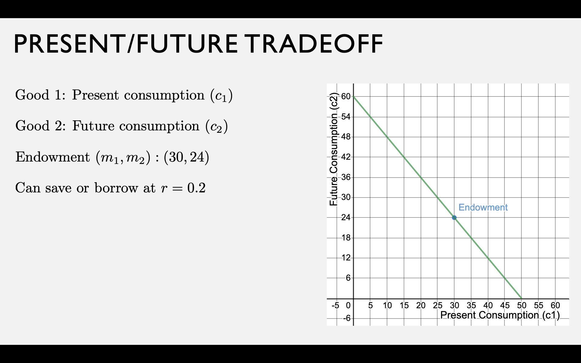
Present-Future Tradeoff
Your endowment is an income stream of \(m_1\) dollars now and \(m_2\) dollars in the future.
What happens if you don't consume all \(m_1\) of your present income?
Two "goods" are present consumption \(c_1\) and future consumption \(c_2\).
c_1 = m_1 - s
c_2 = m_2 + s
Let \(s = m_1 - c_1\) be the amount you save.
Saving and Borrowing with Interest
If you save at interest rate \(r\),
for each dollar you save today,
you get \(1 + r\) dollars in the future.
You can either save some of your current income, or borrow against your future income.
If you borrow at interest rate \(r\),
for each dollar you borrow today,
you have to repay \(1 + r\) dollars in the future.
c_1 = m_1 - s
c_2 = m_2 + (1+r)s
c_2 = m_2 + (1+r)(m - c_1)
(1+r)c_1 + c_2 = (1+r)m_1 + m_2
c_1 = m_1 + b
c_2 = m_2 - (1+r)b
c_2 = m_2 - (1+r)(c_1 - m_1)
(1+r)c_1 + c_2 = (1+r)m_1 + m_2
(1+r)c_1 + c_2 = (1+r)m_1 + m_2
How much can you consume in the future if you save all your present income \(m_1\)?
How much can you consume in the present if you borrow the maximum amount against your future income?
FV = c_2 = (1+r)m_1 + m_2
\displaystyle{PV = c_1 = m_1 + {m_2 \over 1 + r}}
c_1 + \frac{c_2}{1+r} = m_1 + \frac{m_2}{1 + r}
"Present Value"
c_1 + \frac{c_2}{1.2} = 30 + \frac{24}{1.2}
c_1 + \frac{c_2}{1.2} = 50
Preferences
Preferences over Time
u(c_1,c_2) = v(c_1)+\beta v(c_2)
v(c) = \text{“within-period" utility}
\beta = \text{“between-period" discount factor}
v(c) = \ln c
v(c) = c
u(c_1,c_2) = \ln c_1 + \beta \ln c_2
Examples:
v(c) = \sqrt{c}
u(c_1,c_2) = c_1 + \beta c_2
u(c_1,c_2) = \sqrt{c_1} + \beta \sqrt{c_2}
When to borrow and save?
u(c_1,c_2) = v(c_1)+\beta v(c_2)
MRS \text{ at endowment }= {v^\prime (m_1) \over \beta v^\prime (m_2)}
Save if MRS at endowment < \(1 + r\)
Borrow if MRS at endowment > \(1 + r\)
(high interest rates or low MRS)
(low interest rates or high MRS)
If we assume \(v(c)\) exhibits diminishing marginal utility:
MRS is higher if you have less money today (\(m_1\) is low)
and/or more money tomorrow (\(m_2\) is high)
MRS is lower if you are more patient (\(\beta\) is high)
u(c_1,c_2) = v(c_1)+\beta v(c_2)
MRS \text{ at endowment }= {v^\prime (m_1) \over \beta v^\prime (m_2)}
Save if MRS at endowment < \(1 + r\)
Borrow if MRS at endowment > \(1 + r\)
pollev.com/chrismakler

MRS(c_1,c_2) = {c_2 \over \beta c_1}
\text{Example: }v(c_t) = \ln c_t
u(c_1,c_2) = \ln c_1 + \beta \ln c_2
If \(m_1 = 30\), \(m_2 = 24\), and \(\beta = 0.5\),
what is the highest interest rate at which you would borrow money?
Borrow or Save?
MRS(c_1,c_2) = {c_2 \over \beta c_1}
\text{MRS at endowment } =
\text{Price Ratio } =
\text{Example: }v(c_t) = \ln c_t \Rightarrow u(c_1,c_2) = \ln c_1 + \beta \ln c_2
m_1 = 30, m_2 = 24, \beta = 0.5
\text{Generic }m_1,m_2,r
\text{Borrow if } :
MRS(m_1,m_2) = {m_2 \over \beta m_1}
MRS(30,24) = {24 \over 0.5 \times 30}
1 + r
= 1.6
>
1 + r
1.6
>
1 + r
MRS
r < 0.6
1 + r
Optimal Choice
Optimal Bundle
\text{Example: }v(c_t) = \ln c_t \Rightarrow u(c_1,c_2) = \ln c_1 + \beta \ln c_2
Tangency condition:
Budget line:
MRS(c_1,c_2) = {c_2 \over \beta c_1}
{c_2 \over \beta c_1} = 1 + r
(1 + r)c_1 + c_2 = (1 + r)m_1 + m_2
\Rightarrow c_2 = (1+r)\beta c_1
(1 + r)c_1 + (1+r)\beta c_1 = (1 + r)m_1 + m_2
c_1^* = {1 \over 1 + \beta}(m_1 + {m_2 \over 1 + r})
c_2^* = {\beta \over 1 + \beta}((1 + r)m_1 + m_2)
If \(m_1 = 30\), \(m_2 = 24\), \(\beta = 0.25\), and \(r = 0.2\),
what is your optimal choice?
pollev.com/chrismakler
Optimal Bundle
\text{Example: }v(c_t) = \ln c_t \Rightarrow u(c_1,c_2) = \ln c_1 + \beta \ln c_2
Tangency condition:
Budget line:
m_1 = 30, m_2 = 24, \beta = 0.25, r = 0.2
{c_2 \over \beta c_1} = 1 + r
{c_2 \over 0.25 c_1} = 1.2
(1 + r)c_1 + c_2 = (1 + r)m_1 + m_2
1.2c_1 + c_2 = 1.2 \times 30 + 24
1.2c_1 + c_2 = 60
\Rightarrow c_2 = 0.3 c_1
\Rightarrow c_2 = (1+r)\beta c_1
(1 + r)c_1 + (1+r)\beta c_1 = (1 + r)m_1 + m_2
1.2c_1 + 0.3 c_1 = 60
c_1^* = {1 \over 1 + \beta}(m_1 + {m_2 \over 1 + r})
c_2^* = {\beta \over 1 + \beta}((1 + r)m_1 + m_2)
c_1^* = 40
Since you start with \(m_1 = 30\), this means you borrow 10.
MRS(c_1,c_2) = {c_2 \over \beta c_1}
Supply and Demand
Supply of Savings and
Demand for Borrowing
Gross demand = your optimal bundle given interest rate \(r = (c_1^*(r), c_2^*(r))\)
If you want to consume more than your present income at interest rate \(r\),
your demand for borrowing is
\(b(r) = c_1^*(r) - m_1\)
How does this compare to your initial income stream \((m_1,m_2)\)?
If you want to consume less than your present income at interest rate \(r\),
your supply of savings is
\(s(r) = m_1 - c_1^*(r)\)
Different Interest Rates
MRS > 1 + r
MRS < 1 + r
BORROW
SAVE
What if the interest rate is different for borrowing and saving?

c_2 = m_2 + (1 + r)(m_1 - c_1)
Inflation and Real Interest Rates
Suppose there is inflation,
so that each dollar saved can only buy
\(1/(1 + \pi)\) of what it originally could:
c_2 = m_2 + \left({1 + r\over 1 + \pi}\right)(m_1 - c_1)
Up to now, we've been just looking at
dollar amounts in both periods
\text{let }\rho = {1 + r \over 1 + \pi} - 1
c_2 = m_2 + (1 + \rho)(m_1 - c_1)
We call \(r\) the "nominal interest rate" and \(\rho\) the "real interest rate"
For low values of \(r\) and \(\pi\), \(\rho \approx r - \pi\)
c_1 + \frac{c_2}{1+r} = m_1 + \frac{m_2}{1 + r}
"Present Value" for two periods
Beyond Two Periods
If you save \(s\) now, you get \(x = s(1 + r)\) next period.
The amount you have to save in order to get \(x\) one period in the future is
s(1 + r) = x
s = {x \over 1 + r}
Remember how we got this...
If you save \(s\) now, you get \(x = s(1 + r)\) next period.
The amount you have to save in order to get \(x\) one period in the future is
s(1 + r) = x
s = {x \over 1 + r}
If you save for two periods, it grows at interest rate \(r\) again, so \(x_2 = (1+r)(1+r)s = (1+r)^2s\)
Therefore, the amount you have to save in order to get \(x_2\) two periods in the future is
s(1 + r)^2 = x_2
s = {x_2 \over (1 + r)^2}
If you save for two periods, it grows at interest rate \(r\) again, so \(x_2 = (1+r)(1+r)s = (1+r)^2s\)
Therefore, the amount you have to save in order to get \(x_2\) two periods in the future is
s(1 + r)^2 = x_2
s = {x_2 \over (1 + r)^2}
If you save for \(t\) periods, it grows at interest rate \(r\) each period, so \(x_t = (1+r)^ts\)
Therefore, the amount you have to save in order to get \(x_t\), \(t\) periods in the future, is
s(1 + r)^t = x_t
s = {x_t \over (1 + r)^t}
Therefore, the amount you have to save in order to get \(x_t\), \(t\) periods in the future, is
s(1 + r)^t = x_t
s = {x_t \over (1 + r)^t}
We call this the present value of a payoff of \(x_t\)
PV(x_t) = {x_t \over (1 + r)^t}
Application: Social Cost of Carbon
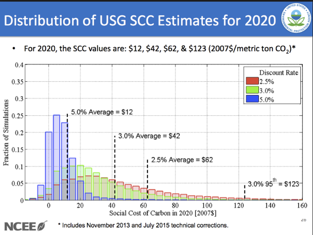
Obama Admin: $45
Uses a 3% discount rate; includes global costs
Trump Admin: less than $6
Uses a 7% discount rate; only includes American costs
PV of $1 Trillion in 2100:
$86B for Obama, $4B for Trump
Econ 50 | Spring 25 | Lecture 19
By Chris Makler
Econ 50 | Spring 25 | Lecture 19
We apply the framework of consumer choice theory to the choice of how to allocation money across time, investigating saving and borrowing.


