Christopher Makler
Stanford University Department of Economics
Econ 51: Lecture 5
Productive Efficiency
We've been starting with an ‟endowment" of goods...

We've been starting with an ‟endowment" of goods...
....but where did this "endowment" come from?
We've been starting with an ‟endowment" of goods...
Today we will look at production decisions and extend our notion of equilibrium to include production, trade, and consumption.
Productive Efficiency
Allocative Efficiency
You cannot reallocate goods
and make someone better off
without making someone else worse off.
You cannot reallocate resources
and produce more of one good
without making less of another good.
This week
Today: Productive Efficiency
- Resources constraints and the PPF
- Opportunity Cost and the Marginal Rate of Transformation (MRT)
- Productive Efficiency with Two Producers: Joint PPFs
- Comparative Advantage
- Prices and Productive Efficiency
Thursday: Competitive Equilibrium
- Joint Supply at Market Prices
- Joint Demand at Market Prices
- Equilibrium
- Gains from Specialization and Trade
- Concluding thoughts
Scarcity and Choice
Economics is the study of how
we use scarce resources
to satisfy our unlimited wants
Resources
Goods
Happiness
🌎
⌚️
🤓

Multiple Uses of Resources
Labor
Fish
🐟
Coconuts
🥥
[GOOD 1]
⏳
[GOOD 2]
L_1
L_2
\overline L
Resource Constraint
L_1
L_2
L_1 + L_2 = \overline L
\overline L
\overline L
\text{Total labor available }=\overline L
y_1 = f_1(L_1)
y_2 = f_2(L_2)
Note: we'll use \(y_1\) and \(y_2\) for the quantities of each good you produce, and \(x_1\) and \(x_2\) for quantities consumed.
This is new notation (thought it's how Varian does it)...not all graphs/notes have been updated with this notation
Production Possibilities
\text{Fish }(y_1)
\text{Coconuts }(y_2)
Resource Constraint
L_1
L_2
L_1 + L_2 = \overline L
\overline L
\overline L
\text{Total labor available }=\overline L
\text{(Good 1 - Good 2 space)}
y_1 = f_1(L_1)
y_2 = f_2(L_2)
f_1(\overline L)
f_2(\overline L)
Example:
\overline L = 12
f_1(L_1) = 2L_1
f_2(L_2) = L_2
RESOURCE CONSTRAINT
PRODUCTION FUNCTIONS
Example:
\overline L = 12
f_1(L_1) = 2L_1
f_2(L_2) = L_2
RESOURCE CONSTRAINT
PRODUCTION FUNCTIONS
How do we draw the PPF?
Method 1: Plot points
L_1
L_2
0
12
6
6
12
0
y_1
0
y_2
12
12
24
6
0
\text{Fish }(y_1)
\text{Coconuts }(y_2)
6
12
18
24
0
0
6
12
18
24
Example:
\overline L = 12
f_1(L_1) = 2L_1
f_2(L_2) = L_2
RESOURCE CONSTRAINT
PRODUCTION FUNCTIONS
How do we draw the PPF?
Method 2: Derive equation
\text{Fish }(y_1)
\text{Coconuts }(y_2)
6
12
18
24
0
0
6
12
18
24
L_1 + L_2 = 12
y_1 = 2L_1
Want to write in terms of \(y_1\) and \(y_2\)...
y_2 = L_2
L_1 = \tfrac{1}{2}y_1
L_2 = y_2
\tfrac{1}{2}y_1 + y_2 = 12
Slope of the PPF:
Marginal Rate of Transformation (MRT)
Rate at which one good may be “transformed" into another
...by reallocating resources from one to the other.
Opportunity cost of producing an additional unit of good 1,
in terms of good 2
Note: we will generally treat this as a positive number
(the magnitude of the slope), just like with did with MRS and the price ratio.
\overline L = 12
f_1(L_1) = 2L_1
f_2(L_2) = L_2
RESOURCE CONSTRAINT
PRODUCTION FUNCTIONS
\text{Fish }(y_1)
\text{Coconuts }(y_2)
6
12
18
24
0
0
6
12
18
24
\tfrac{1}{2}y_1 + y_2 = 12
Finding the MRT
\displaystyle{MRT = \left|{dy_2 \over dy_1}\right| = {1 \over 2}}
It takes \({1 \over 2}\) of an hour (30 minutes)
to make another
unit of good 1
It takes 1 hour to make another
unit of good 2
If you spend 30 more minutes to make another unit of good 1, how much good 2 could you have made in that same 30 minutes?
Suppose we're allocating 3 hours of labor to fish (good 1),
and 9 to coconuts (good 2).
Now suppose we shift
one hour of labor
from coconuts to fish.
How many fish do we gain?
\Delta_2
\Delta_1
9
8
6
8
How many coconuts do we lose?
\Delta_2 = MP_{L_2} = 1\text{ coconut}
\Delta_1 = MP_{L_1} = 2\text{ fish}
\left|\text{slope}\right| = \frac{MP_{L_2}}{MP_{L_1}}
Relationship between MPL's and MRT
f_1(L_1) = 2L_1
f_2(L_2) = L_2
Fish production function
Coconut production function
Resource Constraint
L_1 + L_2 = 150
PPF
pollev.com/chrismakler

Suppose Chuck can use labor
to produce fish (good 1)
or coconuts (good 2).
If we plot his PPF in good 1 - good 2 space, what are the units of Chuck's MRT?
Curved PPFs
If the MPL's are constant, the MRT is constant.
If the MPL's are changing, the MRT is changing as well.
MRT = {MP_{L2} \over {MP_{L1}}}
f_1(L_1) = 2L_1
f_2(L_2) = L_2
MP_{L1} = 2
MP_{L2} = 1
MRT = {MP_{L2} \over {MP_{L1}}}={1 \over 2}
MRT = {MP_{L2} \over {MP_{L1}}}=\sqrt{L_1 \over 12L_2}
f_1(L_1) = \sqrt{12L_1}
f_2(L_2) = \sqrt{L_2}
MP_{L1} = \sqrt{3 \over L_1}
MP_{L2} = \sqrt{1 \over 4L_2}
Two Agents
\overline L = 12
f_1(L_1) = 2L_1
f_2(L_2) = L_2
CHUCK
\overline L = 12
f_1(L_1) = 3L_1
f_2(L_2) = 3L_2
WILSON
DEFINITIONS
Absolute advantage: the ability to produce a good using fewer resources.
Comparative advantage: the ability to produce a good at a lower opportunity cost.
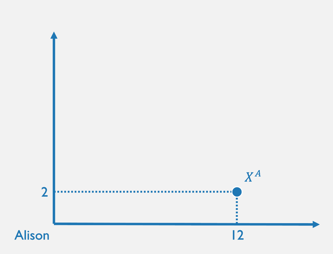
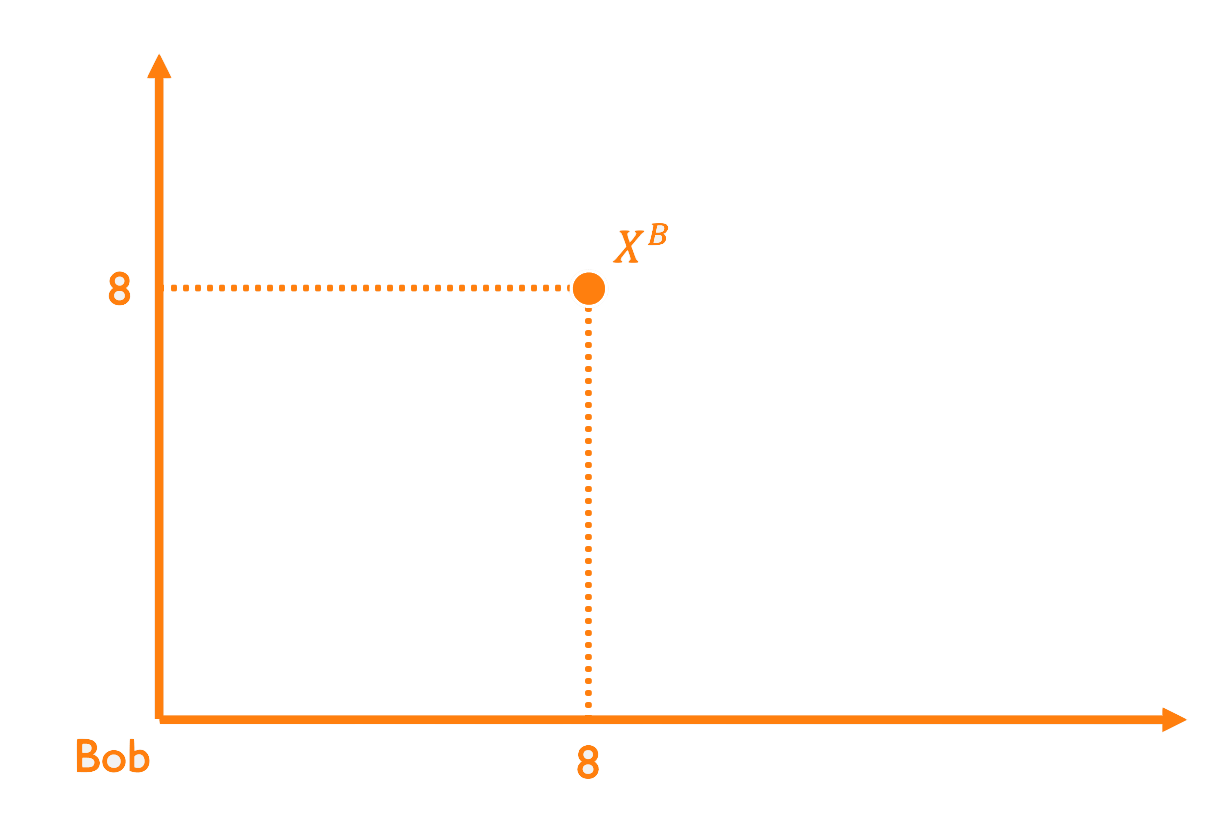
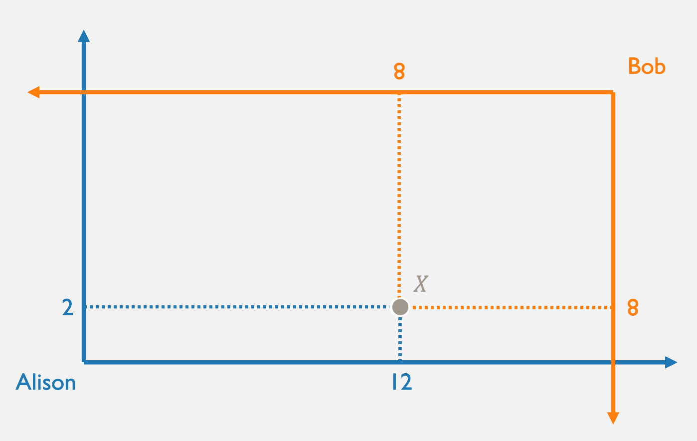
How to construct a joint PPF
- Start from the vertical intercept: its value is the quantity produced of good 2 if everyone completely specializes in good 2.
- As you increase good 1, think about who should produce each unit of the good.
- Continue until you hit the horizontal axis, at the point where everyone specializes in good 1.
- (It's pretty simple with two people and linear PPFs, but there are more complicated ones...)
Joint PPFs with Diminishing MPL
Alison
Bob
MRT = {MP_{L2} \over {MP_{L1}}}=\sqrt{L_1 \over 12L_2}
f_1(L_1) = \sqrt{12L_1}
f_2(L_2) = \sqrt{L_2}
MP_{L1} = \sqrt{3 \over L_1}
MP_{L2} = \sqrt{1 \over 4L_2}
MRT = {MP_{L2} \over {MP_{L1}}}=\sqrt{L_1 \over 2L_2}
f_1(L_1) = \sqrt{12L_1}
f_2(L_2) = \sqrt{6L_2}
MP_{L1} = \sqrt{3 \over L_1}
MP_{L2} = \sqrt{3 \over 2L_2}
Optimal Choice with Prices
Now suppose Chuck can buy and sell these goods at prices \(p_1\) and \(p_2\).
\text{Monetary value of }(y_1,y_2)=p_1y_1 + p_2y_2
Money from spending
another hour producing fish
Money from spending
another hour
producing coconuts
MP_{L1}
\times
p_1
MP_{L2}
\times
p_2
Key Insight:
Money from spending
another hour producing fish
Money from spending
another hour
producing coconuts
MP_{L1}
\times
p_1
MP_{L2}
\times
p_2
You should produce more good 1 if
MP_{L1} \times p_1 > MP_{L2} \times p_2
{p_1 \over p_2} > {MP_{L2} \over MP_{L1}}
pollev.com/chrismakler
Suppose Chuck can produce 2 fish per hour or
1 coconut per hour.
If he can sell
fish at \(p_1 = 3\)
and coconuts at \(p_1 = 4\),
what should he produce?
Big Picture
- Productive efficiency means you can't reallocate resources and make more of both goods
- The joint PPF shows combinations of outputs agents can produce that are productively efficient.
- If agents can sell their goods at market prices, they (collectively) produce at a point along the joint PPF.
Econ 51 | 05 | Comparative Advantage
By Chris Makler
Econ 51 | 05 | Comparative Advantage
Comparative Advantage and the Gains from Trade


