Trading from an Endowment
Christopher Makler
Stanford University Department of Economics
Econ 51: Lecture 3
Today's Agenda
Review: Budget Lines
Review: Optimization Subject to a Budget Line
Endowment Budget Lines
Optimization from an Endowment
Net Demand/Supply
Intertemporal Budget Lines
Demand for Borrowing
Optimal Intertemporal Choice
Review: (Gross) Demand
PART I: REVIEW OF ECON 50
BUDGET LINES DETERMINED BY INCOME
PART II: BUDGET LINES DETERMINED BY AN ENDOWMENT OF GOODS
PART III: BUDGET LINES DETERMINED BY AN INCOME STREAM
[CONSTRAINTS]
[OPTIMIZATION PROBLEM]
[COMPARATIVE STATICS]
MOST IMPORTANT FOR THURSDAY
Part I: Econ 50 Review
Good 1 - Good 2 Space
Two "Goods" : Good 1 and Good 2
\text{Bundle }X\text{ may be written }(x_1,x_2)
x_1 = \text{quantity of good 1 in bundle }X
x_2 = \text{quantity of good 2 in bundle }X
A = (40, 160)
B = (80,80)
\text{Examples:}

\(A\)
\(B\)
Prices
\(A\)
\(B\)
Let's assume all goods have a single, constant price associated with them;
so every unit of good 1 costs \(p_1\)
and every unit of good 2 costs \(p_2\)
Monetary value (cost) of bundle \(X = (x_1,x_2)\):
p_1x_1 + p_2x_2
If \(p_1 = 2\) and \(p_2 = 1\), what is the cost of bundle \(A = (40,160)\)?
What is the cost of bundle \(B = (80,80)\) at those prices?
m = \text{money income}
p_1 = \text{price of good 1}
p_2 = \text{price of good 2}
\text{horizontal intercept} = \frac{m}{p_1}
\text{vertical intercept} = \frac{m}{p_2}
\text{slope of budget line} = -\frac{p_1}{p_2}
Budget Constraints
\text{Example: } p_1 = 2, p_2 = 1, m = 240
\(A\)
\(B\)
We can write down the set of all points that have the same monetary value; in Econ 50 these were "budget constraints" or sometimes "isocost lines."
Spend all $240 on good 1
Spend all $240 on good 2
Equation of line: \(2x_1 + x_2 = 240\)
= \frac{240}{2} = 120
= \frac{240}{1} = 240
More generally,
equation of the budget line: \(p_1x_1 + p_2x_2 = m\)
= -\frac{2}{1} =-2
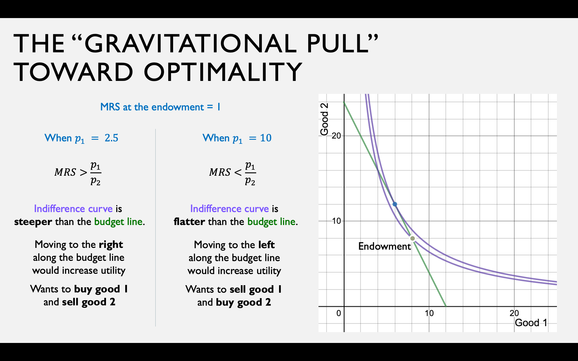
MRS > \frac{p_1}{p_2}
MRS < \frac{p_1}{p_2}
Indifference curve is
steeper than the budget line
Indifference curve is
flatter than the budget line
Moving to the right
along the budget line
would increase utility
Moving to the left
along the budget line
would increase utility
More willing to give up good 2
than the market requires
Less willing to give up good 2
than the market requires
The “Gravitational Pull" Towards Optimality
IF...
THEN...
The consumer's utility function is "well behaved" -- smooth, strictly convex, and strictly monotonic
The indifference curves do not cross the axes
The budget line is a simple straight line
The optimal consumption bundle will be characterized by two equations:
MRS = \frac{p_1}{p_2}
p_1x_1 + p_2x_2 = m
More generally: the optimal bundle may be found using the Lagrange method
Optimal Choice
Otherwise, the optimal bundle may lie at a corner,
a kink in the indifference curve, or a kink in the budget line.
No matter what, you can use the "gravitational pull" argument!
- Write an equation for the tangency condition.
- Write an equation for the budget line.
- Solve for \(x_1^*\) or \(x_2^*\).
- Plug value from (3) into either equation (1) or (2).
u(x_1,x_2) = x_1x_2

Solving for Optimality when Calculus Works
p_1 = 2, p_2 = 1, m = 240
x_1^*(p_1,p_2,m)
x_2^*(p_1,p_2,m)
(Gross) demand functions are mathematical expressions
of endogenous choices as a function of exogenous variables (prices, income).
(Gross) Demand Functions
u(x_1,x_2) = x_1x_2
p_1x_1 + p_2x_2 = m
x_1^*(p_1,p_2,m) = \frac{a}{a+b}\times \frac{m}{p_1}
For a Cobb-Douglas utility function of the form
Special Case: The “Cobb-Douglas Rule"
u(x_1,x_2) = x_1^ax_2^b
The demand functions will be
x_2^*(p_1,p_2,m) = \frac{b}{a+b}\times \frac{m}{p_2}
That is, the consumer will spend fraction \(a/(a+b)\) of their income on good 1, and fraction \(b/(a+b)\) of their income on good 2.
This shortcut is very much worth memorizing! We'll use it a lot in the next few weeks in place of going through the whole optimization process.
pollev.com/chrismakler

Find the optimal bundle for the Cobb-Douglas utility function is
u(x_1,x_2) = \ln x_1 + \tfrac{1}{4} \ln x_2
and the budget constraint is
1.2 x_1 + x_2 = 60
Part II: Endowment Optimization
Trading from an Endowment
Good 1
Good 2
e_2
e_1
E
Note: lots of different notation for the endowment bundle!
Varian uses \(\omega\), some other people use \(x_1^E\)
x_2
x_1
X
Suppose you'd like to move from that endowment to some other bundle X
You start out with some endowment E
This involves trading some of your good 1 to get some more good 2
\Delta x_1
\Delta x_2
\Delta x_1 = e_1 - x_1
\Delta x_2 = x_2 - e_2
Buying and Selling
Good 1
Good 2
e_2
e_1
E
x_2
x_1
X
If you can't find someone to trade good 1 for good 2 directly, you could sell some of your good 1 and use the money to buy good 2.
Suppose you sell \(\Delta x_1\) of good 1 at price \(p_1\). How much money would you get?
Suppose you wanted to buy \(\Delta x_2\) of good 2 at price \(p_2\). How much would that cost?
p_1 \Delta x_1
p_2 \Delta x_2
\Delta x_1
\Delta x_2
\Delta x_1 = e_1 - x_1
\Delta x_2 = x_2 - e_2
=
p_1 (e_1 - x_1)
=
p_2 (x_2 - e_2)
Buying and Selling
Good 1
Good 2
e_2
e_1
E
x_2
x_1
X
\Delta x_1
\Delta x_2
\Delta x_1 = e_1 - x_1
\Delta x_2 = x_2 - e_2
p_1 (e_1 - x_1)
=
p_2 (x_2 - e_2)
If the amount you get from selling good 1 exactly equals the amount you spend on good 2, then
p_2x_2 - p_2e_2 = p_1e_1 - p_1x_1
p_1x_1 + p_2x_2 = p_1e_1 +p_2e_2
monetary value of \(E\)
at market prices
monetary value of \(X\)
at market prices
(Basically: you can afford any bundle with the same monetary value as your endowment.)
Endowment Budget Line
Good 1
Good 2
e_2
e_1
E
p_1x_1 + p_2x_2 = p_1e_1 +p_2e_2
If you sell all your good 1 for \(p_1\),
how much good 2 can you consume?
If you sell all your good 2 for \(p_2\),
how much good 1 can you consume?
If \(x_1 = 0\):
If \(x_2 = 0\):
x_2 = e_2 + {p_1e_1 \over p_2}
x_1 = e_1 + {p_2e_2 \over p_1}
Endowment Budget Line
Good 1
Good 2
e_2
e_1
E
p_1x_1 + p_2x_2 = p_1e_1 +p_2e_2
e_2 + {p_1e_1 \over p_2}
e_1 + {p_2e_2 \over p_1}
Liquidation value of your endowment
\hat m
Divide both sides by \(p_2\):
{p_1 \over p_2}x_1 + x_2 = {p_1 \over p_2} e_1 + e_2
{\hat m \over p_2} =
Divide both sides by \(p_1\):
x_1 + {p_2 \over p_1}x_2 = e_1 + {p_2 \over p_1}e_2
{\hat m \over p_1} =
In other words: the endowment budget line is just like a normal budget line,
but the amount of money you have is the liquidation value of your endowment.
Endowment Budget Line
p_1x_1+p_2x_2=p_1e_1+p_2e_2
Divide both sides by \(p_2\):
Divide both sides by \(p_1\):
The budget line only depends on the price ratio \({p_1 \over p_2}\),
not the individual prices.
{p_1 \over p_2}x_1 + x_2 = {p_1 \over p_2} e_1 + e_2
x_1 + {p_2 \over p_1}x_2 = e_1 + {p_2 \over p_1}e_2
Effect of a Change in Prices
What happens if the price of good 1 doubles?
What happens if both prices double?


pollev.com/chrismakler
Bob has an endowment of (8,8) and can buy and sell goods 1 and 2. What happens to his endowment budget line if the price of good 1 decreases? You may select more than one answer.

Optimization
Optimization problem with money
Optimization problem with an endowment
\displaystyle{\max_{x_1,x_2}\ u(x_1,x_2)}
\text{s.t. }p_1x_1 + p_2x_2 = m
\displaystyle{\max_{x_1,x_2}\ u(x_1,x_2)}
\text{s.t. }p_1x_1 + p_2x_2 = p_1e_1+p_2e_2
Procedure is exactly the same - we just have a different equation for the budget constraint.


pollev.com/chrismakler
Bob has the endowment (8,8) and the utility function $$u(x_1,x_2)=x_1x_2$$If he faces prices \(p_1 = 10\) and \(p_2 = 5\), what is his optimal choice?
Optimization: Income vs. Endowment
Recall: The “Gravitational Pull" Argument
Before, it was a thought experiment: "What if you were to buy bundle X? Would you have preferred to move to the right?"
Now, you actually are at some bundle like X, and are deciding to trade left or right along your budget line.
pollev.com/chrismakler
Suppose Alison has the endowment (12,2) and the utility function $$u(x_1,x_2)=x_1x_2$$ If the price of good 2 is 6, for what price of good 1 will she be willing to sell some of her good 1?


Gross Demands and Net Demands
The total quantity of a good
you want to consume (i.e. end up with)
at different prices.
Gross Demand
The transaction you want to engage in
(the amount you want to buy or sell)
at different prices.
Net Demand
x_1^*(p_1,p_2,e_1,e_2)
x_1^*(p_1,p_2,e_1,e_2) - e_1


\text{Net demand: }ND(p_1,p_2) = x_1^*(p_1,p_2) - e_1
Is this positive or negative?
Positive: you are a net demander of good 1.
Negative: you are a net supplier of good 1.
d_1(p_1 | p_2) = \begin{cases} 0 & \text{ if } x_1^\star(p_1,p_2) \le e_1\\x_1^\star(p_1,p_2) - e_1 & \text{ if } x_1^\star(p_1,p_2) \ge e_1\end{cases}
s_1(p_1 | p_2) = \begin{cases}e_1 - x_1^\star(p_1,p_2) & \text{ if } x_1^\star(p_1,p_2) \le e_1 \\ 0 & \text{ if } x_1^\star(p_1,p_2) \ge e_1\end{cases}
It's a little confusing that economists use the terms "net demand" to mean
both the general difference between what you want and where you are,
and the specific case in which you demand more of a good. Sorry. :(
MOST IMPORTANT FOR THURSDAY
Part II: Most Important Takeaways
The endowment budget line depends only on the price ratio, not on individual prices.
Whether you're a net demander or supplier depends on the relationship between the price ratio and the MRS at the endowment.
Budget Line
Present-Future Tradeoff
Your endowment is an income stream of \(m_1\) dollars now and \(m_2\) dollars in the future.
What happens if you don't consume all \(m_1\) of your present income?
Two "goods" are present consumption \(c_1\) and future consumption \(c_2\).
c_1 = m_1 - s
c_2 = m_2 + s
Let \(s = m_1 - c_1\) be the amount you save.
Saving and Borrowing with Interest
If you save at interest rate \(r\),
for each dollar you save today,
you get \(1 + r\) dollars in the future.
You can either save some of your current income, or borrow against your future income.
If you borrow at interest rate \(r\),
for each dollar you borrow today,
you have to repay \(1 + r\) dollars in the future.
c_1 = m_1 - s
c_2 = m_2 + (1+r)s
c_2 = m_2 + (1+r)(m - c_1)
(1+r)c_1 + c_2 = (1+r)m_1 + m_2
c_1 = m_1 + b
c_2 = m_2 - (1+r)b
c_2 = m_2 - (1+r)(c_1 - m_1)
(1+r)c_1 + c_2 = (1+r)m_1 + m_2
(1+r)c_1 + c_2 = (1+r)m_1 + m_2
INTERTEMPORAL BUDGET LINE
ENDOWMENT BUDGET LINE
p_1x_1 + p_2x_2 = p_1e_1 + p_2e_2
What is the slope?
What does it represent?
Lecture 1: Preferences over Time
u(c_1,c_2) = v(c_1)+\beta v(c_2)
v(c) = \text{“within-period" utility}
\beta = \text{“between-period" discount factor}
v(c) = \ln c
u(c_1,c_2) = \ln c_1 + \beta \ln c_2
Example: Cobb-Douglas Utility
MRS = {v'(c_1) \over \beta v'(c_2)}
MRS(c_1,c_2)={c_2 \over \beta c_1}
When to borrow and save?
u(c_1,c_2) = v(c_1)+\beta v(c_2)
MRS \text{ at endowment }= {v^\prime (m_1) \over \beta v^\prime (m_2)}
Save if MRS at endowment < \(1 + r\)
Borrow if MRS at endowment > \(1 + r\)
(high interest rates or low MRS)
(low interest rates or high MRS)
If we assume \(v(c)\) exhibits diminishing marginal utility:
MRS is higher if you have less money today (\(m_1\) is low)
and/or more money tomorrow (\(m_2\) is high)
MRS is lower if you are more patient (\(\beta\) is high)
u(c_1,c_2) = \ln(c_1)+\beta \ln(c_2)
MRS \text{ at endowment }= {m_2 \over \beta m_1}
Save if MRS at endowment < \(1 + r\)
Borrow if MRS at endowment > \(1 + r\)
pollev.com/chrismakler
MRS(c_1,c_2) = {c_2 \over \beta c_1}
If \(m_1 = 30\), \(m_2 = 24\), and \(\beta = 0.5\),
what is the highest interest rate at which you would borrow money?
Borrow or Save?
MRS(c_1,c_2) = {c_2 \over \beta c_1}
\text{MRS at endowment } =
\text{Price Ratio } =
\text{Example: }v(c_t) = \ln c_t \Rightarrow u(c_1,c_2) = \ln c_1 + \beta \ln c_2
m_1 = 30, m_2 = 24, \beta = 0.5
\text{Generic }m_1,m_2,r
\text{Borrow if } :
MRS(m_1,m_2) = {m_2 \over \beta m_1}
MRS(30,24) = {24 \over 0.5 \times 30}
1 + r
= 1.6
>
1 + r
1.6
>
1 + r
MRS
r < 0.6
1 + r
Optimal Bundle
\text{Example: }v(c_t) = \ln c_t \Rightarrow u(c_1,c_2) = \ln c_1 + \beta \ln c_2
Tangency condition:
Budget line:
MRS(c_1,c_2) = {c_2 \over \beta c_1}
{c_2 \over \beta c_1} = 1 + r
(1 + r)c_1 + c_2 = (1 + r)m_1 + m_2
\Rightarrow c_2 = (1+r)\beta c_1
(1 + r)c_1 + (1+r)\beta c_1 = (1 + r)m_1 + m_2
c_1^* = {1 \over 1 + \beta}(m_1 + {m_2 \over 1 + r})
c_2^* = {\beta \over 1 + \beta}((1 + r)m_1 + m_2)
If \(m_1 = 30\), \(m_2 = 24\), \(\beta = 0.25\), and \(r = 0.2\),
what is your optimal choice?
pollev.com/chrismakler
Optimal Bundle
\text{Example: }v(c_t) = \ln c_t \Rightarrow u(c_1,c_2) = \ln c_1 + \beta \ln c_2
Tangency condition:
Budget line:
m_1 = 30, m_2 = 24, \beta = 0.25, r = 0.2
{c_2 \over \beta c_1} = 1 + r
{c_2 \over 0.25 c_1} = 1.2
(1 + r)c_1 + c_2 = (1 + r)m_1 + m_2
1.2c_1 + c_2 = 1.2 \times 30 + 24
1.2c_1 + c_2 = 60
\Rightarrow c_2 = 0.3 c_1
\Rightarrow c_2 = (1+r)\beta c_1
(1 + r)c_1 + (1+r)\beta c_1 = (1 + r)m_1 + m_2
1.2c_1 + 0.3 c_1 = 60
c_1^* = {1 \over 1 + \beta}(m_1 + {m_2 \over 1 + r})
c_2^* = {\beta \over 1 + \beta}((1 + r)m_1 + m_2)
c_1^* = 40
Since you start with \(m_1 = 30\), this means you borrow 10.
MRS(c_1,c_2) = {c_2 \over \beta c_1}
Demand for borrowing:
MOST IMPORTANT FOR THURSDAY
Supply of savings:
d_1(r) = c_1^*(r) - m_1
s_1(r) = m_1 - c_1^*(r)
(when \(MRS(m_1,m_2) > 1 + r\) )
(when \(MRS(m_1,m_2) < 1 + r\) )
c_2 = m_2 + (1 + r)(m_1 - c_1)
Bonus: Inflation and Real Interest Rates
Suppose there is inflation,
so that each dollar saved can only buy
\(1/(1 + \pi)\) of what it originally could:
c_2 = m_2 + \left({1 + r\over 1 + \pi}\right)(m_1 - c_1)
Up to now, we've been just looking at
dollar amounts in both periods
\text{let }\rho = {1 + r \over 1 + \pi} - 1
c_2 = m_2 + (1 + \rho)(m_1 - c_1)
We call \(r\) the "nominal interest rate" and \(\rho\) the "real interest rate"
For low values of \(r\) and \(\pi\), \(\rho \approx r - \pi\)
Econ 51 | 03 | Trading from an Endowment
By Chris Makler
Econ 51 | 03 | Trading from an Endowment
Building the Basis of Exchange Equilibrium


