Course Retrospective
Christopher Makler
Stanford University Department of Economics
Econ 50: Lecture 25
Plan for the Week
- Wednesday lecture: review
- Wednesday Q section: review
- No other sections
- SEA study hall: tonight 6:30-8:30, Lathrop 282
- Office hours (rotating cast of TA's, me): 10am-6pm Thursday, Lathrop 292
Ways to Think about Learning
Strategic:
"knowing when" - given an unstructured problem, which model/framework is most relevant?
Schematic:
Procedural:
Declarative:
"knowing why" - how do different concepts/models relate to one other?
"knowing how" - given a well-defined problem, ability to follow correct procedure to solve it
"knowing that" - facts and figures, vocabulary
Goals of the Course
Strategic:
Develop rigorous approach to economic modeling; understand how assumptions map into conclusions.
Schematic:
Procedural:
Declarative:
Understand the relationships between
words, math, and graphs.
Learn the techniques of
optimization, equilibrium, and comparative statics.
Know the definitions of key economic terms.
Two Kinds of Optimization
Tradeoffs between two goods
Optimal quantity of one good
🍎
(not feasible)
(feasible)
🍌
Optimal choice
🙂
😀
😁
😢
🙁
🍎
benefit and cost per unit
Marginal Cost
Marginal Benefit
Optimal choice
Two Kinds of Optimization
Tradeoffs between two goods
Optimal quantity of one good
- Modeling consumer preferences
with multivariate calculus - Utility maximization subject to a budget constraint
- Consumer demand
Midterm 1: April 25
- Cost minimization
- Firm profit maximization and supply
- Competitive equilibrium
Midterm 2: May 16
Model: Consumer Choice
Models: Firms, Markets
Remaining 2-3 weeks: real-world applications of these models
Today's Agenda
- Constrained optimization with
more than one choice variable - Unconstrained optimization with
one choice variable - Comparative statics
Modules 1-4, Module 7
Analyzing Tradeoffs
Choices in general
Choices of commodity bundles
Choosing bundles of two goods
Good 1 \((x_1)\)
Good 2 \((x_2)\)
Completeness axiom:
any two bundles can be compared.
Implication: given any bundle \(A\),
the choice space may be divided
into three regions:
preferred to A
dispreferred to A
indifferent to A
Indifference curves cannot cross!
A
The indifference curve through A connects all the bundles indifferent to A.
Indifference curve
through A
Special Case: Good 1 - Good 2 Space
Good 1 - Good 2 Space
What tradeoff is represented by moving
from bundle A to bundle B?
ANY SLOPE IN GOOD 1 - GOOD 2 SPACE
IS MEASURED IN
UNITS OF GOOD 2 PER UNIT OF GOOD 1
ANY SLOPE IN GOOD 1 - GOOD 2 SPACE
IS MEASURED IN
UNITS OF GOOD 2 PER UNIT OF GOOD 1
TW: HORRIBLE STROBE EFFECT!
Marginal Rate of Substitution
🍏🍏
🍏🍏
🍏🍏
🍏🍏
🍏🍏
🍌🍌🍌🍌
🍌🍌🍌🍌
🍌🍌🍌🍌
🍌🍌🍌🍌
🍌🍌🍌🍌
🍌🍌🍌🍌
🍏🍏
🍏🍏
🍏🍏
🍏🍏
🍏🍏
🍏🍏
🍌🍌🍌🍌
🍌🍌🍌🍌
🍌🍌🍌🍌
🍌🍌🍌🍌
🍌🍌🍌🍌
Suppose you were indifferent between the following two bundles:
Starting at bundle X,
you would be willing
to give up 4 bananas
to get 2 apples
Let apples be good 1, and bananas be good 2.
Starting at bundle Y,
you would be willing
to give up 2 apples
to get 4 bananas
Visually: the MRS is the magnitude of the slope
of an indifference curve
Calculating the MRS
Along an indifference curve, all bundles will produce the same amount of utility
In other words, each indifference curve
is a level set of the utility function.
The slope of an indifference curve is the MRS. By the implicit function theorem,
UTILS
UNITS OF GOOD 1
UTILS
UNITS OF GOOD 2
Intertemporal choice: \(c_1\), \(c_2\) represent
consumption in different time periods.
Risk aversion: \(c_1\), \(c_2\) represent
consumption in different states of the world.
Applications from Module 7
If \(v(c)\) exhibits diminishing marginal utility:
MRS is higher if you have less money today
and/or more money tomorrow
MRS is lower if you are more patient (\(\beta\) is high)
MRS is higher if state 1 is more likely to occur
(\(\pi\) is higher)
Let \(v(c)\) be the value function describing how much utility you get from money/consumption
Modeling preferences with functional forms


PERFECT
SUBSTITUTES
PERFECT
COMPLEMENTS
INDEPENDENT
PERFECT
SUBSTITUTES
Constant Elasticity of Substitution (CES) Utility
[50Q only]
- A change in the price of a good results in a movement along its demand curve
- A change in income or the price of other goods results in a shift of the demand curve
Risk aversion
Choice space:
all possible options
Feasible set:
all options available to you
Optimal choice:
Your best choice(s) of the ones available to you
Constrained Optimization
One type of feasible set: the budget set
Prices and Expenditure
Suppose each good has a constant price
(so every unit of the good costs the same)
Budget Line
How much can you consume in the future if you save all your present income \(m_1\)?
How much can you consume in the present if you borrow the maximum amount against your future income?
Selling Labor at a Constant Wage
Leisure (R)
Consumption (C)
You sell \(L\) hours of labor at wage rate \(w\).
You start with 24 hours of leisure and \(M\) dollars.
You earn \(\Delta C = wL\) dollars in addition to the \(M\) you had.
...and you consume \(R = 24 - L\) hours of leisure.
Budget Line Equation
Leisure (R)
Consumption (C)
How does this compare to a normal budget line?
You sell \(L\) hours of labor at wage rate \(w\).
You start with 24 hours of leisure and \(M\) dollars.
You earn \(\Delta C = wL\) dollars in addition to the \(M\) you had.
...and you consume
\(R = 24 - L\) hours of leisure.
Combining preferences and constraints
If we superimpose the budget line on the utility "hill" the nature of the problem becomes clear:
Question: mathematically, how does the utility change as you spend more money on good 1?
What does it mean if you get more "bang for your buck" from good 1 than good 2?
The consumer receives more utility per additional unit of good 1 than the price reflects, relative to good 2.
The consumer receives more
"bang for the buck"
(utils per dollar)
from good 1 than good 2.
Regardless of how you look at it, the consumer would be
better off moving to the right along the budget line --
i.e., consuming more of good 1 and less of good 2.
The consumer is more willing to give up good 2
to get good 1
than the market requires.
IF...
THEN...
The consumer's preferences are "well behaved"
-- smooth, strictly convex, and strictly monotonic
\(MRS=0\) along the horizontal axis (\(x_2 = 0\))
The budget line is a simple straight line
The optimal consumption bundle will be characterized by two equations:
More generally: the optimal bundle may be found using the Lagrange method
\(MRS \rightarrow \infty\) along the vertical axis (\(x_1 \rightarrow 0\))
The Lagrange Method
Cost of Bundle X
Income
Utility
The Lagrange Method
Income left over
Utility
The Lagrange Method
Income left over
Utility
(utils)
(dollars)
utils/dollar
First Order Conditions
"Bang for your buck" condition: marginal utility from last dollar spent on every good must be the same!
The Lagrange Method
Utility Maximization
Cost Minimization
Solution functions:
"Ordinary" Demand functions
Solution functions:
"Compensated" Demand functions
Utility Maximization
Cost Minimization
Utility Maximization
Cost Minimization
Solution functions:
"Ordinary" Demand functions
Solution functions:
"Compensated" Demand functions
What is the optimized value of the objective function?
INDIRECT UTILITY FUNCTION
EXPENDITURE FUNCTION
Utility from utility-maximizing choice,
given prices and income
Cost of cost-minimizing choice,
given prices and a target utility
Utility Maximization
Cost Minimization
What is the optimized value of the objective function?
INDIRECT UTILITY FUNCTION
EXPENDITURE FUNCTION
The Lagrange Method: Utility Maximization
Income left over
Utility
(utils)
(dollars)
utils/dollar
The Lagrange Method: Consumer Cost Minimization
Expenditure
Utility
(utils)
(dollars)
dollars/util
The Lagrange Method: Consumer Cost Minimization
Expenditure
Utility
(utils)
(dollars)
dollars/util
The Lagrange Method: Firm Cost Minimization
Cost
Output
(units)
(dollars)
dollars/unit
Firm Cost Minimization
First Order Conditions
MRTS (slope of isoquant) is equal to the price ratio
What happens when the Lagrange method fails?
- Corner solutions
- Solutions at kinks
Interior Solution:
Corner Solution:
Optimal bundle contains
strictly positive quantities of both goods
Optimal bundle contains zero of one good
(spend all resources on the other)
If only consume good 1: \(MRS \ge {p_1 \over p_2}\) at optimum
If only consume good 2: \(MRS \le {p_1 \over p_2}\) at optimum
Corner Solutions
\(MRS < {p_1 \over p_2}\) along
the entire budget line!

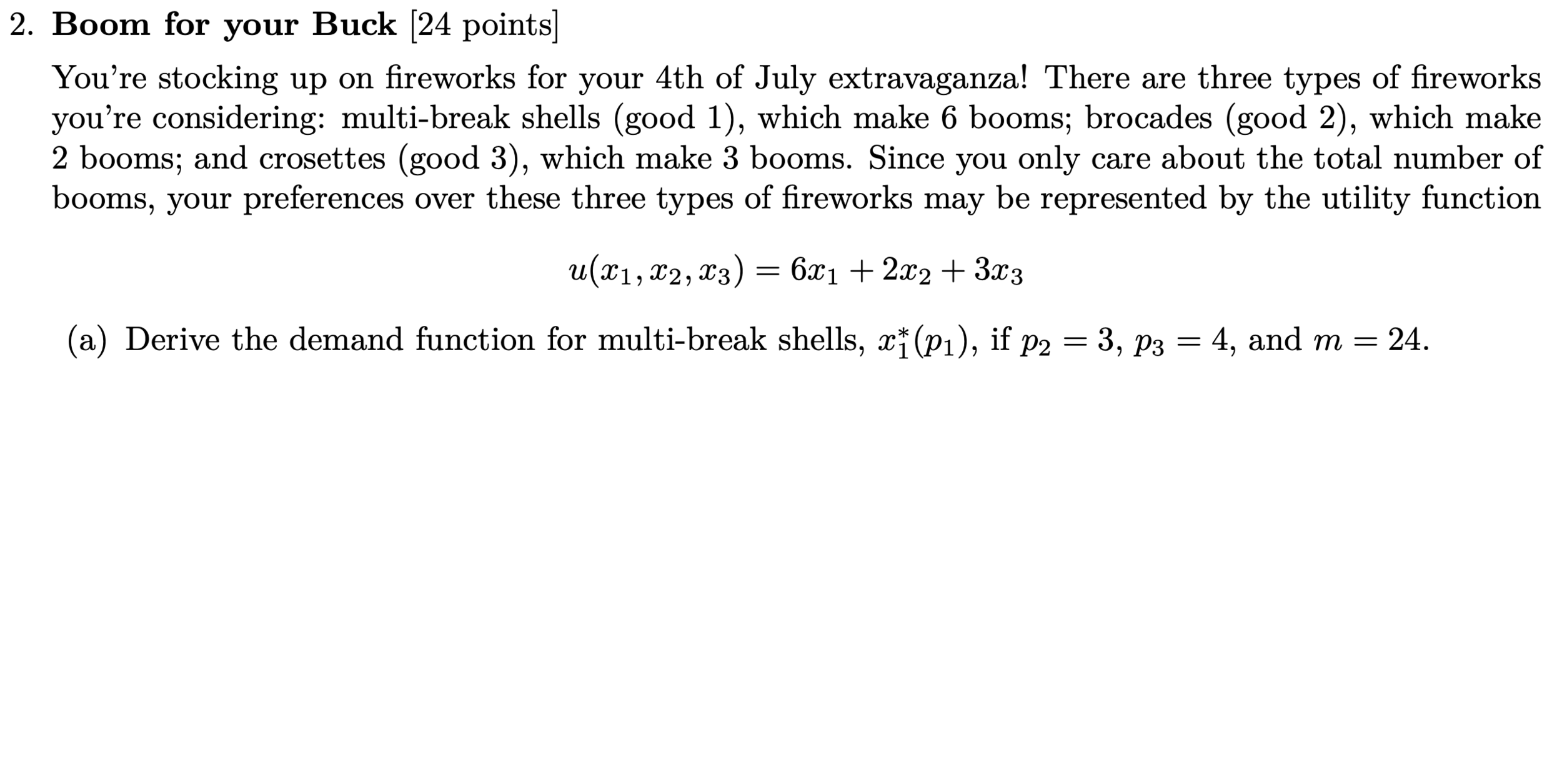
Key insight: you will only buy the good with the highest "boom for the buck" (i.e., \(MU/p\)).
What does this tell us about goods 2 and 3?
You will never buy good 2!

Key insight: you will only buy the good with the highest "boom for the buck" (i.e., \(MU/p\)).
When will you only buy good 1?

Key insight: you will only buy the good with the highest "boom for the buck" (i.e., \(MU/p\)).
When will you only buy good 1?

Key insight: you will only buy the good with the highest "boom for the buck" (i.e., \(MU/p\)).
What happens if you try to equate the MU/p across goods (or equivalently, set the MRS's equal to the price ratios)?
How to Solve a Kinked Constraint Problem
- Evaluate the MRS at the kink
- Compare it to the price ratio on either side of the kink
- If \(MRS > {p_1 \over p_2}\) to the right of the kink, the solution is to the right of the kink; use the equation for that line and maximize.
- If \(MRS < {p_1 \over p_2}\) to the left of the kink, the solution is to the left of the kink; use the equation for that line and maximize.
- If the MRS is between the price ratios, then the solution is at the kink.
- Note: if the price ratio to the left of the kink is greater than the price ratio to the left, it's more complicated...you could have two potential solutions! Maximize subject to each of the constraints and compare utility at the respective maxima.
Summary: Constrained Optimization
- Analysis of tradeoffs
- Lagrange multiplier represents the "exchange rate" between the units of the objective function and the units of the constraint.
- Lagrange method works by equating "bang for your buck" (or "buck for your bang" / marginal cost) across competing goods.
- However, some solutions occur at corners or kinks where bang for your buck is not equated; in that case, have to apply logic.
Today's Agenda
- Constrained optimization with
more than one choice variable - Unconstrained optimization with
one choice variable - Comparative statics
✅
How much of a good to produce?
- Firm: maximize profit by setting MR(q) = MC(q)
- Competitive firm: maximize profit by setting P = MC(q)
- Market: maximize sum of consumer and producer surplus by setting D(p) = S(p)
- Market with externalities, common resources: maximize social welfare by setting MSB = MSC
- Public goods: maximize social welfare by setting the sum of marginal benefits equal to marginal cost
Theory of the Firm
Labor
Firm
🏭
Capital
⏳
⛏
Customers
🤓
Firms buy inputs
and produce some good,
which they sell to a customer.
PRICE
QUANTITY
Labor
Capital
Output
Firm
🏭
Costs
Revenue
Theory of the Firm
Firms buy inputs
and produce some good,
which they sell to a customer.
PRICE
QUANTITY
Labor
Capital
Output
Costs
Revenue
Profit
The difference between their revenue and their cost is what we call profits, denoted by the Greek letter \(\pi\).
Theory of the Firm
Costs
Revenue
Profit
Theory of the Firm
Our approach will be to write costs, revenues, and profits all as functions of the ouput \(q\).
Pigovian tax:
Internalize the externality so that private marginal cost equals social marginal cost.
Competitive equilibrium:
consumers set \(P = MB\),
producers set \(P = PMC \Rightarrow MB = PMC\)
With a tax: consumers set \(P = MB\),
producers set \(P - t = PMC\)
Fees
Suppose you needed to buy a fishing permit for a fee F.
What value of F would result in the optimal L*?
Taxes
Suppose the village levied a tax of t per fish caught.
What value of t would result in the optimal L*?
Solving for the Optimal Quantity
- Figure out the profit or welfare function from the context of the question; write this as a function of the relevant choice variable
- Take the derivative and set it equal to zero!
- Be able to interpret this as balancing the relevant marginal benefits and marginal costs.
Today's Agenda
- Constrained optimization with
more than one choice variable - Unconstrained optimization with
one choice variable - Comparative statics
✅
✅
Optimization: What is the optimal bundle for a given situation?
Comparative Statics: What happens to the optimal bundle when something about that situation changes?
🍏
🍌
BL1
Example: solve for the optimal bundle
as a function of income and prices:
The solutions to this problem will be called the demand functions. We have to think about how the optimal bundle will change when \(p_1,p_2,m\) change.
BL2
- A change in the price of a good results in a movement along its demand curve
- A change in income or the price of other goods results in a shift of the demand curve
Analyzing Comparative Statics
- Solve the optimization problem as a function of the variables that will shift the solution
- Try to determine if there are key points where behavior changes
- Know how to tell a story with a graph: most times, you don't have to graph things precisely, just show how a change percolates graphically through a model!
Summary
- Relatively few mathematical techniques
- Lots of different applications
- Within each application, know your definitions well so you can apply the relevant techniques.
- Read the questions carefully, think before you write, and don't do too much work: most questions can be answered without solving for an optimum.
- Good luck!
Econ 50 | Spring 25 | Lecture 25
By Chris Makler
Econ 50 | Spring 25 | Lecture 25
Course Retrospective
- 1,249


