The Marginal Rate of Substitution and the Implicit Function Theorem
Christopher Makler
Stanford University Department of Economics
Econ 50: Lecture 3
Today's Agenda
- Thinking about tradeoffs: the marginal rate of substitution (MRS)
- Derivatives of multivariate functions and the Implicit Function Theorem
- Applying the IFT to the MRS

Math
Econ
previously in Econ 50...
Choices in general
Choices of commodity bundles
Choosing bundles of two goods
Good 1 \((x_1)\)
Good 2 \((x_2)\)
Given any bundle \(A\),
the choice space may be divided
into three regions:
preferred to A
dispreferred to A
indifferent to A
A
The indifference curve through A connects all the bundles indifferent to A.
Indifference curve
through A
Good 1 - Good 2 Space
Good 1 - Good 2 Space
x_1
x_2
Two "Goods" (e.g. apples and bananas)
A bundle is some quantity of each good
\text{Bundle }X = (x_1,x_2)
x_1 = \text{quantity of good 1 in bundle }X
x_2 = \text{quantity of good 2 in bundle }X
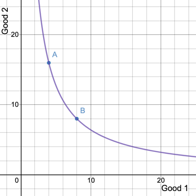
Can plot this in a graph with \(x_1\) on the horizontal axis and \(x_2\) on the vertical axis
A = (4,16)
B = (8,8)
A
B
4
8
12
16
20
4
8
12
16
20
Good 1 - Good 2 Space
x_1
x_2
What tradeoff is represented by moving
from bundle A to bundle B?
\text{Give up }\Delta x_2 =
A
B
4
8
12
16
20
4
8
12
16
20
\text{Gain }\Delta x_1 =
\text{Rate of exchange }=
ANY SLOPE IN GOOD 1 - GOOD 2 SPACE
IS MEASURED IN
UNITS OF GOOD 2 PER UNIT OF GOOD 1
ANY SLOPE IN GOOD 1 - GOOD 2 SPACE
IS MEASURED IN
UNITS OF GOOD 2 PER UNIT OF GOOD 1
TW: HORRIBLE STROBE EFFECT!
8 \text{ units of good 2}
4 \text{ units of good 1}
2
\displaystyle{\frac{\text{units of good 2}}{\text{units of good 1}}}
\Delta x_2
\Delta x_1
Marginal Rate of Substitution
X = (10,24)
🍏🍏
🍏🍏
🍏🍏
🍏🍏
🍏🍏
🍌🍌🍌🍌
🍌🍌🍌🍌
🍌🍌🍌🍌
🍌🍌🍌🍌
🍌🍌🍌🍌
🍌🍌🍌🍌
Y=(12,20)
🍏🍏
🍏🍏
🍏🍏
🍏🍏
🍏🍏
🍏🍏
🍌🍌🍌🍌
🍌🍌🍌🍌
🍌🍌🍌🍌
🍌🍌🍌🍌
🍌🍌🍌🍌
Suppose you were indifferent between the following two bundles:
Starting at bundle X,
you would be willing
to give up 4 bananas
to get 2 apples
Let apples be good 1, and bananas be good 2.
Starting at bundle Y,
you would be willing
to give up 2 apples
to get 4 bananas
MRS = {4 \text{ bananas} \over 2 \text{ apples}}
= 2\ {\text{bananas} \over \text{apple}}
Visually: the MRS is the magnitude of the slope
of an indifference curve
How do we calculate the MRS from a utility function?
Let's review what we learned last time
about multivariable functions...
Multivariable Functions
x
f()
z = f(x,y)
y
z
[INDEPENDENT VARIABLES]
[DEPENDENT VARIABLE]
\text{Level set for }z=\{(x,y)|f(x,y)=z\}
Derivative of a Univariate Function
at a point \(x\)
{dy \over dx} = \lim_{\Delta x \rightarrow 0}\frac{f(x + \Delta x) - f(x)}{\Delta x}
the height of the function changes
per distance traveled to the right
rate at which
\displaystyle{{df \over dx} = \lim_{\Delta x \rightarrow 0} {f(x + \Delta x) - f(x) \over \Delta x}}
Local Linearization
{dy \over dx} = \lim_{\Delta x \rightarrow 0}\frac{f(x + \Delta x) - f(x)}{\Delta x}
\approx \frac{\Delta y}{\Delta x}

c(q) = 10q + q^2
Example: suppose a firm's cost function is given by
Suppose the firm is already producing \(q = 30\) units of output. Approximately how much would it cost to produce three more?
{dy \over dx}
\frac{\Delta y}{\Delta x} \approx
\Delta y \approx \Delta x \times {dy \over dx}
Example:
c(q) = 10q + q^2
MC(q) = {dc \over dq} = 10 + 2q
\begin{aligned}
c(30) &= 10 \times 30 + 30^2 = 1,200\\
c(33) &= 10 \times 33 + 33^2 = 1,419
\end{aligned}
\Delta c = 219
MC(30) = {dc \over dq} = 10 + 2 \times 30 = 70
Pretty close to \(3 \times 70\)!
Local Linearization
Partial Derivatives of a Multivariate Function
at a point \((x,y)\)
{\partial f \over \partial x} = \lim_{\Delta x \rightarrow 0}\frac{f(x + \Delta x,y) - f(x,y)}{\Delta x}
{\partial f \over \partial y} = \lim_{\Delta y \rightarrow 0}\frac{f(x,y + \Delta y) - f(x,y)}{\Delta y}
the height of the function changes
per distance traveled East
rate at which
the height of the function changes
per distance traveled North
rate at which
\displaystyle{{\partial f \over \partial x} = \lim_{\Delta x \rightarrow 0} {f(x + \Delta x, y) - f(x, y) \over \Delta x}}
\displaystyle{{\partial f \over \partial y} = \lim_{\Delta y \rightarrow 0} {f(x, y + \Delta y) - f(x, y) \over \Delta y}}
Univariate Chain Rule
\text{Example: }h(x)=(3x + 2)^2
h(x)=f(g(x))
{dh \over dx} = {df \over dg} \times {dg \over dx}
f(g)=g^2
g(x)=3x+2
Multivariable Chain Rule
\text{Example: }h(x,y)=(3x+y)^2
h(x,y)=f(g(x,y))
{\partial h \over \partial x} = {df \over dg} \times {\partial g \over \partial x}
f(g)=g^2
g(x)=3x+y
y(x)=4-0.4x
Total Derivative Along a Path
\text{How does }f(x,y)\text{ change along a path?}
\Delta f \approx
\displaystyle{{\partial f \over \partial x} \times \Delta x}
\displaystyle{{\partial f \over \partial y} \times \Delta y}
+
\text{Suppose the path is defined by some function }y(x):
\Delta f \approx
\displaystyle{{\partial f \over \partial x} \times \Delta x}
\displaystyle{{\partial f \over \partial y}}
+
\displaystyle{\times {dy \over dx}}
\displaystyle{\times \Delta x}
\displaystyle{\Delta f \over \Delta x} \approx
\displaystyle{{\partial f \over \partial x}}
\displaystyle{{\partial f \over \partial y}}
+
\displaystyle{\times {dy \over dx}}
Total Derivative Along a Path
\displaystyle{\Delta f \over \Delta x}\ \ \ \ \ \ \approx
\displaystyle{{\partial f \over \partial x}}
\displaystyle{{\partial f \over \partial y}}
+
\displaystyle{\times\ \ \ \ \ \ {dy \over dx}}
The total change in the height of the function due to a small increase in \(x\)
The amount \(f\) changes due to the increase in \(x\)
[indirect effect through \(y\)]
The amount \(f\) changes due to an increase in \(y\)
The amount \(y\) changes due to an increase in \(x\)
[direct effect from \(x\)]
Derivative Along a Level Set
f(x,y)=z
Take total derivative of both sides with respect to x:
Solve for \(dy/dx\):
\displaystyle{{\partial f \over \partial x}}
\displaystyle{{\partial f \over \partial y}}
+
\displaystyle{\times \ \ {dy \over dx}}
=
0
\displaystyle{{dy \over dx}}
= -
\displaystyle{{\partial f \over \partial x}}
\displaystyle{{\partial f \over \partial y}}
IMPLICIT FUNCTION THEOREM
Derivative Along a Level Set
f(x,y)=z
Total derivative with respect to x:
\displaystyle{{\partial f \over \partial x}}
\displaystyle{{\partial f \over \partial y}}
+
\displaystyle{\times \ \ {dy \over dx}}
=
0
2x + 4y = 20
2
4
+
\displaystyle{\times \ \ {dy \over dx}}
=
0
=
-2
\displaystyle{{dy \over dx}}
= -
\displaystyle{{\partial f \over \partial x}}
\displaystyle{{\partial f \over \partial y}}
IMPLICIT FUNCTION THEOREM
\displaystyle{{dy \over dx}}
= -
2
4
4
\displaystyle{\times \ \ {dy \over dx}}
pollev.com/chrismakler
Consider the multivariable function
f(x,y) = 4x^{1 \over 2}y
What is the slope of the level set passing through the point (1, 5)?

ECONOMICS
Application to Utility Functions: Marginal Utility
MU_1(x_1,x_2) = {\partial u(x_1,x_2) \over \partial x_1}
MU_2(x_1,x_2) = {\partial u(x_1,x_2) \over \partial x_2}
Given a utility function \(u(x_1,x_2)\),
we can interpret the partial derivatives
as the "marginal utility" from
another unit of either good:
UTILS
UNITS OF GOOD 1
UTILS
UNITS OF GOOD 2
Indifference Curves and the MRS
Along an indifference curve, all bundles will produce the same amount of utility
In other words, each indifference curve
is a level set of the utility function.
The slope of an indifference curve is the MRS. By the implicit function theorem,
MRS(x_1,x_2) = \frac{\partial u(x_1,x_2) \over \partial x_1}{\partial u(x_1,x_2) \over \partial x_2} = {MU_1 \over MU_2}
UTILS
UNITS OF GOOD 1
UTILS
UNITS OF GOOD 2
Indifference Curves and the MRS
Along an indifference curve, all bundles will produce the same amount of utility
In other words, each indifference curve
is a level set of the utility function.
The slope of an indifference curve is the MRS. By the implicit function theorem,
MRS(x_1,x_2) = \frac{\partial u(x_1,x_2) \over \partial x_1}{\partial u(x_1,x_2) \over \partial x_2} = {MU_1 \over MU_2}
UNITS OF GOOD 1
UNITS OF GOOD 2
If you give up \(\Delta x_2\) units of good 2, how much utility do you lose?
If you get \(\Delta x_1\) units of good 1, how much utility do you gain?
\Delta u \approx \Delta x_2 \times MU_2
\Delta u \approx \Delta x_1 \times MU_1
If you end up with the same utility as you begin with:
\Delta x_2 \times MU_2 \approx \Delta x_1 \times MU_1
{\Delta x_2 \over \Delta x_1} \approx {MU_1 \over MU_2}
pollev.com/chrismakler
What is the MRS of the utility function \(u(x_1,x_2) = x_1x_2\)?
\displaystyle{MRS = {MU_1 \over MU_2} =}
u(x_1,x_2) = x_1x_2
\displaystyle{MU_1 = {\partial u(x_1,x_2) \over \partial x_1} =}
\displaystyle{MU_2 = {\partial u(x_1,x_2) \over \partial x_2} =}
4 \times 16
A = (4,16)
B = (8,8)
8 \times 8
x_2
x_1
\displaystyle{x_2 \over x_1}
= 64
= 64
16
8
4
8
\displaystyle{16 \over 4}
=4
\displaystyle{8 \over 8}
=1
MRS = 4
MRS = 1
Example: draw the indifference curve for \(u(x_1,x_2) = \frac{1}{2}x_1x_2^2\) passing through (4,6).
Step 1: Evaluate \(u(x_1,x_2)\) at the point
Step 2: Set \(u(x_1,x_2)\) equal to that value.
Step 4: Plug in various values of \(x_1\) and plot!
\(u(4,6) = \frac{1}{2}\times 4 \times 6^2 = 72\)
\(\frac{1}{2}x_1x_2^2 = 72\)
\(x_2^2 = \frac{144}{x}\)
\(x_2 = \frac{12}{\sqrt x_1}\)
How to Draw an Indifference Curve through a Point: Method I
Step 3: Solve for \(x_2\).
How would this have been different if the utility function were \(u(x_1,x_2) = \sqrt{x_1} \times x_2\)?
\(u(4,6) =\sqrt{4} \times 6 = 12\)
\(\sqrt{x_1} \times x_2 = 12\)
\(x_2 = \frac{12}{\sqrt x_1}\)
Example: draw the indifference curve for \(u(x_1,x_2) = \frac{1}{2}x_1x_2^2\) passing through (4,6).
Step 1: Derive \(MRS(x_1,x_2)\). Determine its characteristics: is it smoothly decreasing? Constant?
Step 2: Evaluate \(MRS(x_1,x_2)\) at the point.
Step 4: Sketch the right shape of the curve, so that it's tangent to the line at the point.
How to Draw an Indifference Curve through a Point: Method II
Step 3: Draw a line passing through the point with slope \(-MRS(x_1,x_2)\)
How would this have been different if the utility function were \(u(x_1,x_2) = \sqrt{x_1} \times x_2\)?
\text{In both cases }MRS(x_1,x_2) = \frac{MU_1(x_1,x_2)}{MU_2(x_1,x_2)} = \frac{x_2}{2x_1}
MRS(4,6) = \frac{6}{2 \times 4} = \frac{3}{4}
This is continuously strictly decreasing in \(x_1\) and continuously strictly increasing in \(x_2\),
so the function is smooth and strictly convex and has the "normal" shape.
Summary
MRS(x_1,x_2) = \frac{\partial u(x_1,x_2) \over \partial x_1}{\partial u(x_1,x_2) \over \partial x_2} = {MU_1 \over MU_2}
UNITS OF GOOD 1
UNITS OF GOOD 2
\text{Along the level set }f(x,y)=z,
\displaystyle{{dy \over dx}}
= -
\displaystyle{{\partial f \over \partial x}}
\displaystyle{{\partial f \over \partial y}}
IMPLICIT FUNCTION THEOREM
The Marginal Rate of Substitution is the magnitude of the slope of an indifference curve; so, by the implicit function theorem:
Econ 50 | Fall 25 | Lecture 03
By Chris Makler
Econ 50 | Fall 25 | Lecture 03
Modeling Production with Multivariate Functions


