Book 2. Quantitative Analysis
FRM Part 1
QA 9. Regression Diagnostics
Presented by: Sudhanshu
Module 1. Heteroskedasticity and Multicollinearity
Module 2. Model Specification
Module 1. Heteroskedasticity and Multicollinearity

Topic 1. Heteroskedasticity and Its Consequences
Topic 2. Detecting and Correcting Heteroskedasticity
Topic 3. Multicollinearity and Its Consequences
Topic 4. Detecting and Correcting Multicollinearity
Topic 1. Heteroskedasticity and Its Consequences
- Definition: A regression exhibits heteroskedasticity when the variance of the residuals (errors) is not constant across observations.
-
Types:
- Unconditional Heteroskedasticity: Random and unrelated to explanatory variables (less concerning).
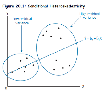
- Conditional Heteroskedasticity: Residual variance increases or decreases systematically with the level of an independent variable.
-
Consequences:
- OLS coefficient estimates remain unbiased and consistent.
-
Standard errors are unreliable, leading to:
- Invalid t-tests and confidence intervals.
- Misleading significance levels.
- Real-World Example: Income data often shows higher variability among high earners.
Topic 1. Heteroskedasticity and Its Consequences
Practice Questions: Q1
Q1. Effects of conditional heteroskedasticity include which of the following problems?
I. The coefficient estimates in the regression model are biased.
II. The standard errors are unreliable.
A. I only.
B. II only.
C. Both I and II.
D. Neither I nor II.
Practice Questions: Q1 Answer
Explanation: B is correct.
Effects of heteroskedasticity include the following:
(1) The standard errors are usually unreliable estimates and
(2) the coefficient estimates are not affected.
Topic 2. Detecting and Correcting Heteroskedasticity
-
Visual Inspection (Using Scatterplot):
- Residual plot vs. X or predicted Y – Look for funnel shapes or patterns.
-
Formal Testing – Breusch-Pagan Test:
-
Step 1: Estimate OLS and compute residuals.
- Step 2: Square the residuals and regress on original Xs.
- Step 3: Compute test statistic:
- Step 4: Compare with chi-squared critical value.
-
Decision:
- If reject null of homoskedasticity → heteroskedasticity is present.
-
-
If conditional heteroskedasticity is detected, we can conclude that the coefficients are unaffected but the standard errors are unreliable. In such a case, revised, White standard errors should be used in hypothesis testing instead of the standard errors from OLS estimation procedures.
-
Correction Method:
- Use White's heteroskedasticity-consistent standard errors.
- These adjust variance estimates, preserving valid hypothesis testing.
\chi^2=n \times R^2
\chi^2>\text { critical }\chi^2,
Practice Questions: Q2
Q2. Der-See Hsu, researcher for Xiang Li Quant Systems, is using a multiple regression model to forecast currency values. Hsu determines that the chi-squared statistics calculated using the of the regression involving the squared residuals as dependent variable exceeds the chi-squared critical value. Which of the following is
the most appropriate conclusion for Hsu to reach?
A. Hsu should estimate the White standard errors for use in hypothesis testing.
B. OLS estimates and standard errors are consistent, unbiased, and reliable.
C. OLS coefficients are biased but standard errors are reliable.
D. A linear model is inappropriate to model the variation in the dependent variable.
R^2
Practice Questions: Q2 Answer
Explanation: A is correct.
Hsu’s test results indicate that the null hypothesis of no conditional
heteroskedasticity should be rejected. In such a case, the OLS estimates of standard errors would be unreliable and Hsu should estimate White corrected standard errors for use in hypothesis testing. Coefficient estimates would still be reliable (i.e., unbiased and consistent).
Topic 3. Multicollinearity and Its Consequences
-
Definition: Occurs when two or more independent variables are highly correlated.
-
Perfect Collinearity: One variable is an exact linear combination of others (violates OLS assumption).
-
Consequences:
-
Coefficient estimates remain unbiased, but:
-
Standard errors increase.
-
t-values decrease, making significant variables appear insignificant.
-
Leads to Type II errors (failing to reject a false null).
-
-
-
Example:
- Including both “Years of Education” and “Highest Degree Level” in a wage model can induce multicollinearity.
Topic 4. Detecting and Correcting Multicollinearity
-
Signs of Multicollinearity:
- High R² and significant F-test, but insignificant t-tests for individual variables.
-
Variance Inflation Factor (VIF):
- R² is from regressing Xj on all other Xs.
- If VIF > 10 (i.e. ), multicollinearity is problematic.
-
Correction Techniques:
- Drop one or more correlated Xs (based on theory or t-values).
- Use Principal Component Analysis (PCA) or stepwise regression to reduce dimensionality.
\mathrm{VIF}_j=\frac{1}{1-R_j^2}
R_j^2>90\%
Practice Questions: Q3
Q3. Ben Strong recently joined Equity Partners as a junior analyst. Within a few weeks, Strong successfully modeled the movement of price for a hot stock using a multiple regression model. Beth Sinclair, Strong’s supervisor, is in charge of evaluating the results of Strong’s model. What is the most appropriate conclusion for Sinclair based
on the variance information factor (VIF) for each of the explanatory variables included in Strong’s model as shown here?
A. Variables X1 and X2 are highly correlated and should be combined into one variable.
B. Variable X3 should be dropped from the model.
C. Variable X2 should be dropped from the model.
D. Variables X1 and X2 are not statistically significant.
\begin{array}{cr}
\hline \text { Variable } & \text { VIF } \\
\hline \text { X1 } & 2.1 \\
\text { X2 } & 10.3 \\
\text { X3 } & 6.9
\end{array}
Practice Questions: Q3 Answer
Explanation: C is correct.
VIF > 10 for independent variable X2 indicates that it is highly correlated with the other two independent variables in the model, indicating multicollinearity. One of the approaches to overcoming the problem of multicollinearity is to drop the highly correlated variable.
Practice Questions: Q4
Q4. Which of the following statements regarding multicollinearity is least accurate?
A. Multicollinearity may be present in any regression model.
B. Multicollinearity is not a violation of a regression assumption.
C. Multicollinearity makes it difficult to determine the contribution to explanation of the dependent variable of an individual explanatory variable.
D. If the t-statistics for the individual independent variables are insignificant, yet the F-statistic is significant, this indicates the presence of multicollinearity.
Practice Questions: Q4 Answer
Explanation: A is correct.
Multicollinearity will not be present in a single regression. While perfect collinearity is a violation of a regression assumption, the presence of multicollinearity is not. Divergence between t-test and F-test is one way to detect the presence of multicollinearity. Multicollinearity makes it difficult to precisely measure the contribution of an independent variable toward explaining the
variation in the dependent variable.
Module 2. Model Specification
Topic 1. Model Specification
Topic 2. Omitted Variable Bias
Topic 3. Bias-Variance Tradeoff
Topic 4. Residual Plots
Topic 5. Identifying Outliers
Topic 6. The Best Linear Unbiased Estimator (BLUE)
Topic 1. Model Specification
- Model Specification: Choosing the correct independent variables and functional form.
-
Issues:
- Omitting relevant variables → biased estimates.
- Including irrelevant variables → reduces adjusted R² and adds noise.
- Good practice: Base model selection on economic theory, prior research, and diagnostic tests.
- Example: Modeling housing prices without accounting for location would miss a key explanatory variable.
Topic 2. Omitted Variable Bias
-
Definition: Omitted variable bias is present when two conditions
are met:
-
the omitted variable is correlated with other independent variables in the model, and
-
the omitted variable is a determinant of the dependent variable.
-
-
Mathematical Impact:
- OLS tries to assign the missing variable's impact to correlated Xs → biased coefficients.
-
Consequences:
- Invalidates inference and prediction.
- Bias does not vanish with a large sample size (unlike variance).
- Example: Excluding “Experience” in a wage regression may inflate the effect of “Education”.
Practice Questions: Q5
Q5. The omitted variable bias results from:
A. exclusion of uncorrelated independent variables.
B. inclusion of uncorrelated independent variables.
C. inclusion of correlated independent variables.
D. exclusion of correlated independent variables.
Practice Questions: Q5 Answer
Explanation: D is correct.
Omitted variable bias results from excluding a relevant independent variable that is correlated with other independent variable.
Topic 3. Bias-Variance Tradeoff
- Bias: Error from oversimplifying a model (e.g., underfitting).
- Variance: Error from overfitting, i.e., too sensitive to training data.
-
Tradeoff:
- Simple models: High bias, low variance.
- Complex models: Low bias, high variance.
- Goal: Minimize total error = bias² + variance + irreducible error.
-
Model Selection Approaches:
- General-to-Specific: Start with full model, drop insignificant variables iteratively.
- m-fold Cross-Validation: Split dataset into m parts, train on m–1, validate on 1, rotate, and average error.
Practice Questions: Q6
Q6. Which of the following statements about bias-variance tradeoff is most accurate?
A. Models with a large number of independent variables tend to have a high bias error.
B. High variance error results when the out-of-sample R2 of a regression is high.
C. Models with fewer independent variables tend to have a high variance error.
D. General-to-specific model is one approach to resolve the bias-variance tradeoff.
Practice Questions: Q6 Answer
Explanation: D is correct.
Larger, overfit models have a low bias error (high in-sample but low out-ofsample). Smaller, parsimonious models have lower
in-sample and a lower variance error. Two ways to resolve the bias-variance tradeoff are the general-to specific model and m-fold cross-validation.
R^2
R^2
R^2
Topic 4. Residual Plots
- Purpose: Diagnose issues in model assumptions.
-
Types:
-
Raw Residual Plot (eᵢ vs ŷ): Non-random pattern may suggest:
- Non-linearity
- Heteroskedasticity
-
Standardized Residuals: Highlights extreme observations.
- Residuals beyond ±2: suspicious
- Residuals beyond ±4: likely outliers
-
Raw Residual Plot (eᵢ vs ŷ): Non-random pattern may suggest:
- Best Practice: Residuals should appear random, centered around zero, and show no pattern.
Topic 5. Identifying Outliers
- Outlier Impact on Regression: Linear regression assumes no outliers in sample data; outliers skew estimated regression parameters and cause large changes in coefficient values when removed
- Cook's Distance Formula: Cook's distance identifies outliers using the following metric:
- where
- = predicted value of y after dropping outlier observation j
- = predicted value of y without dropping any observation
- k = number of residual variables
- = squared residual in the model with all observations
- Interpretation Threshold: Large values of Cook's distance (Dj > 1) indicate the dropped observation is indeed an outlier
\mathrm{D}_{\mathrm{j}}=\frac{\sum_{\mathrm{i}=1}^{\mathrm{n}}\left(\widehat{\mathrm{y}}_i^{(-\mathrm{j})}-\widehat{\mathrm{y}}_{\mathrm{i}}\right)^2}{\mathrm{kS}^2}
S^2
\widehat{\mathrm{y}}_{\mathrm{i}}
\widehat{\mathrm{y}}^{(\mathrm{-j})}
Topic 6. The Best Linear Unbiased Estimator (BLUE)
- Gauss-Markov Theorem: Under classical assumptions, OLS gives the Best Linear Unbiased Estimator (BLUE).
-
Conditions:
- Linearity in parameters
- Random sampling
- No perfect collinearity
- Homoskedasticity
- Uncorrelated residuals
- Zero mean residuals: E(ε) = 0
-
Implication:
- Among all linear and unbiased estimators, OLS has lowest variance.
- Note: Normality of residuals is not required for BLUE, but needed for valid hypothesis testing.
Practice Questions: Q7
Q7. Evaluate the following statements:
I. A high value of Cook’s distance indicates the presence of an outlier.
II. Cook’s distance is inversely related to the squared residuals.
A. Both statements are correct.
B. Only Statement I is correct.
C. Only Statement II is correct.
D. Both statements are incorrect.
Practice Questions: Q7 Answer
Explanation: A is correct.
Both statements are correct. A high value of Cook’s distance for an observation (>1) indicates that it is an outlier. The squared residuals are in the denominator in the computation of Cook’s distance and, hence, are inversely related to the measure.
Copy of QA 9. Regression Diagnostics
By Prateek Yadav


