Book 2. Quantitative Analysis
FRM Part 1
QA 8. Regression with Multiple Explanatory Variables
Presented by: Sudhanshu
Module 1. Multiple Regression
Module 2. Measures of Fit In Linear Regression
Module 1. Multiple Regression

Topic 1. Relative Assumptions of Single and Multiple Regression
Topic 2. Interpreting Multiple Regression Coefficients
Topic 3. Interpreting Multiple Regression Results
Topic 1. Relative Assumptions of Single and Multiple Regression
- Multiple Regression Model:
- : Regression or slope coefficients; sensitivity of Y to changes in (controlling for all other Xs)
- α: Value of Y when all Xs=0
- : Random error or shock; unexplained component of Y.
-
Assumptions of Single Regression (modified for multiple Xs):
- The expected value of the error term, conditional on the independent variables, is zero:
- All (Xs and Y) observations are i.i.d.
- The variance of X is positive (otherwise estimation of β would not be possible).
- The variance of the errors is constant (i.e., homoskedasticity).
- There are no outliers observed in the data.
-
Additional Assumption for Multiple Regression: X variables are not perfectly correlated (i.e., they are not perfectly linearly dependent). Each X variable should have some variation not fully explained by other X variables.
Y=\alpha+\beta_1 X_1+\beta_2 X_2+\ldots+\beta_k X_k+\varepsilon
\beta_j
X_j
[E(\epsilon_i|X_{i's})=0].
\varepsilon
Practice Questions: Q1
Q1. Which of the following is not an assumption of single regression
A. There are no outliers in the data.
B. The variance of the independent variables is greater than zero.
C. Independent variables are not perfectly correlated.
D. Residual variance are homoskedastic.
Practice Questions: Q1 Answer
Explanation: C is correct.
This is an assumption for multiple regression and not for single regression.
Topic 2. Interpreting Multiple Regression Coefficients
- Partial Slope Coefficient Interpretation: In multiple regression, slope coefficients (called partial slope coefficients) capture the change in the dependent variable for a one-unit change in the independent variable, holding other independent variables constant
- OLS Estimation for Multiple Regression: Differs from single regression through a stepwise process where explanatory variables are first regressed against other explanatory variables, and residuals become new explanatory variables
- Two-Independent-Variable Model:
- Step 1 - Estimate Residuals: Regress X₁ against X₂ using OLS (coefficients a and b are not used, only residuals):
- Step 2 - Estimate Residuals: Regress Y against X₂ to obtain residuals:
- Final Step - Calculate β₁: Regress Step 2 residuals against Step 1 residuals to estimate the slope coefficient:
- Controlling for Variation: This stepwise process ensures β₁ is calculated after controlling for variation in X₂; the process can be reversed to estimate β₂ after controlling for X₁
Y_i=\alpha+\beta_1 \times X_{1 i}+\beta_2 \times X_{2 i}+\varepsilon_i
X_{1 i}=a+b \times X_{2 i}+\phi_i
Y_i=c+d \times X_{2 i}+\lambda_i
\lambda_i=\beta_1 \times \phi_i+\varepsilon_i
Practice Questions: Q2
Q2. Multiple regression was used to explain stock returns using the following variables: Dependent variable: RET= annual stock returns (%)
Independent variables: MKT= market capitalization=market capitalization / $1.0 million.
IND= industry quartile ranking (IND = 4 is the highest ranking)
FORT= Fortune 500 firm, where {FORT=1 if the stock is that of a Fortune 500 firm, FORT=0 if not a Fortune 500 stock}
The regression results are presented in the following table.
Based on the results in the table, which of the following most accurately represents the regression equation?
A. 0.43 + 3.09(MKT) + 2.61(IND) + 1.70(FORT).
B. 0.681 + 0.021(MKT) + 0.04(IND) + 0.139(FORT).
C. 0.522 + 0.0460(MKT) + 0.7102(IND) + 0.9(FORT).
D. 1.21 + 0.015(MKT) + 0.2725(IND) + 0.5281(FORT).
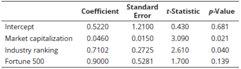
Practice Questions: Q2 Answer
Explanation: C is correct.
The coefficients column contains the regression parameters.
Practice Questions: Q3
Q3. Multiple regression was used to explain stock returns using the following variables:
Dependent variable: RET= annual stock returns (%)
Independent variables:
- MKT= market capitalization=market capitalization/$1.0 million.
- IND= industry quartile ranking (IND = 4 is the highest ranking)
- FORT= Fortune 500 firm, where {FORT=1 if the stock is that of a Fortune 500 firm, FORT=0 if not a Fortune 500 stock}
The regression results are presented in the following table.
The expected amount of the stock return attributable to it being a Fortune 500 stock is closest to:
A. 0.522.
B. 0.046.
C. 0.710.
D. 0.900.
Practice Questions: Q3 Answer
Explanation: D is correct.
The regression equation is 0.522 + 0.0460(MKT) + 0.7102(IND) + 0.9(FORT). The coefficient on FORT is the amount of the return attributable to the stock of a Fortune 500 firm.
- Single Variable Regression: In the regression Y = 2.0 + 4.5X₁, if X₁ increases by 1 unit, Y is expected to increase by 4.5 units
- Adding a Second Variable: When X₂ is added to create Y = 1.0 + 2.5X₁ + 6.0X₂, the slope coefficient for X₁ changes from 4.5 to 2.5
- Why Coefficients Change: Slope coefficients typically change when adding variables unless the new variable (X₂) is uncorrelated with existing variables (X₁)
- When X₁ increases by 1 unit, X₂ is also expected to change
- Multiple regression captures this relationship between X₁ and X₂ when predicting Y
- Multiple Regression Interpretation: In Y = 1.0 + 2.5X₁ + 6.0X₂, if X₁ increases by 1 unit, Y is expected to increase by 2.5 units, holding X₂ constant
- Intercept Interpretation: The intercept (1.0) represents the expected value of Y when all independent variables equal zero
Topic 3. Interpreting Multiple Regression Results
- Example: A researcher estimated the following three-factor model to explain the return on different portfolios (Returns are expressed in percentage form).
- Calculate the following:
-
The return on a portfolio when
-
The impact on portfolio return if declines by 1%
-
The expected return on the portfolio when
-
- Answer:
-
Change in portfolio return
-
when all factors = 0 would be the intercept = 1.70%
Topic 3. Interpreting Multiple Regression Results
R_m=R_z=R_v=0
R_z
\mathrm{R}_{\mathrm{m}}=8 \%, \mathrm{R}_{\mathrm{z}}=2 \% \text { and } \mathrm{R}_{\mathrm{v}}=3 \%
E\left(R_p\right)=1.70+(1.03 \times 8)-(0.23 \times 2)+(0.32 \times 3)=10.44 \%
=\Delta R_P=-(0.23 \times-1)=+0.23 \%
E\left(R_p\right)
R_{P, i}=1.70+1.03 R_{m, i}-0.23 R_{z, i}+0.32 R_{v, i}
Module 2. Measures of Fit in Linear Regression
Topic 1. Components of Total Variation
Topic 2. Coefficient of Determination
Topic 3. Adjusted
Topic 4. Joint Hypothesis Tests and Confidence Intervals
Topic 5. The F-Test
R^2
Topic 1. Components of Total Variation
- Standard Error of the Regression (SER): Measures the uncertainty about the accuracy of predicted values of the dependent variable. A stronger relationship means data points are closer to the regression line (smaller errors).
- OLS Estimation: Minimizes the sum of squared differences between predicted and actual values.
- Decomposition of Total Variation:
- The regression model explains the variation in Y:
- Deviation from mean for Y:
- Therefore:
-
\sum(Y_i -\bar{Y})^2
Y_i-\bar{Y}=(\hat{Y}_i-\bar{Y})+(Y_i-\hat{Y}_i)
\sum(Y_i-\bar{Y})^2=\sum(\hat{Y}_i-\bar{Y})^2+\sum(Y_i-\hat{Y})^2
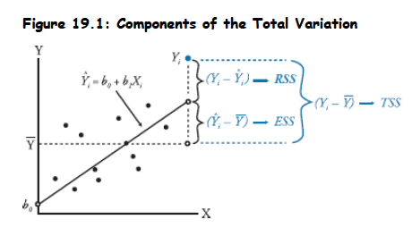
- From above: TSS = ESS + RSS
- TSS=Total Sum of Squares (total variation in Y)
- ESS=Explained Sum of Squares (variation in Y explained by the model)
- RSS=Residual Sum of Squares (unexplained variation in Y)
Topic 2. Coefficient of Determination
- Definition: The coefficient of determination ( ) is the proportion of variation in Y that is explained by the regression model.
- =ESS/TSS=% of variation explained by the regression model
- For multiple regression, is the square of the correlation between Y and the predicted value of Y.
- Limitations of as a sole measure of explanatory power:
- almost always increases as independent variables are added, even if their marginal contribution is not statistically significant. This can lead to overestimating the regression's explanatory power.
- is not comparable across models with different dependent (Y) variables.
- There are no clear predefined values of to indicate if a model is "good." Even low values can provide valuable insight for noisy variables (e.g., currency values)
R^2
R^2
R^2
R^2
R^2
R^2
R^2
R^2
Topic 3. Adjusted
-
To overcome the problem of overestimating the impact of additional variables, researchers recommend adjusting for the number of independent variables.
-
Formula for Adjusted
-
-
- n=number of observations
- k=number of independent variables
-
-
Key Characteristics of Adjusted :
- will always be less than or equal to .
- Adding a new independent variable will increase , but it may either increase or decrease . If the new variable has only a small effect on , may decrease.
- may be less than zero if is low enough.
R^2
R^2
R^2
R^2 (R_a^2):
R_a^2=1-\left[\left(\frac{n-1}{n-k-1}\right)\times (1-R^2)\right]
R^2
R_a^2
R^2
R^2
R_a^2
R^2
R_a^2
R_a^2
R^2
R^2
Topic 3. Adjusted
-
Example 1: An analyst runs a regression of monthly value-stock returns on 5 independent variables over 60 months. The total sum of squares for the regression is 460, and the residual sum of squares is 170. Calculate the and adjusted .
-
Answer 1:
-
-
-
-
The of 63% suggests that the five independent variables together explain 63% of the variation in monthly value-stock returns.
-
- Example 2: Suppose the analyst now adds four more independent variables to the previous regression, and the increases to 65.0%. Identify which model the analyst would most likely prefer.
- Answer 2: With nine independent variables, even though the has increased from 63% to 65%, the adjusted has decreased from 59.6% to 58.7%:
-
The analyst would prefer the first model because the adjusted is higher and the model has five independent variables as opposed to nine.
R^2
\begin{aligned}
& R^2=\frac{460-170}{460}=0.630=63.0 \% \\
& R_a^2=1-\left[\left(\frac{60-1}{60-5-1}\right) \times(1-0.63)\right]=0.596=59.6 \%
\end{aligned}
R^2
R^2
R^2
R^2
R^2
R^2
R_a^2=1-\left[\left(\frac{60-1}{60-9-1}\right) \times(1-0.65)\right]=0.587=58.7 \%
R^2
Practice Questions: Q4
Q4. When interpreting the and adjusted measures for a multiple regression, which of the following statements incorrectly reflects a pitfall that could lead to invalid conclusions?
A. The measure does not provide evidence that the most or least appropriate independent variables have been selected.
B. If the is high, we have to assume that we have found all relevant independent variables.
C. If adding an additional independent variable to the regression improves the , this variable is not necessarily statistically significant.
D. The measure may be spurious, meaning that the independent variables may show a high ; however, they are not the exact cause of the movement in the dependent variable.
R^2
R^2
R^2
R^2
R^2
R^2
R^2
Practice Questions: Q4 Answer
Explanation: B is correct.
If the is high, we cannot assume that we have found all relevant independent variables. Omitted variables may still exist, which would improve the regression results further.
R^2
Topic 4. Joint Hypothesis Tests and Confidence Intervals
-
The magnitude of coefficients does not indicate the importance of independent variables. Hypothesis testing is needed to determine if variables significantly contribute to explaining the dependent variable.
-
t-statistic for Individual Coefficients:
- Degrees of freedom for multiple regression: (n−k−1)
-
Testing Statistical Significance ( versus ):
- Example: Test significance of PR at 10% level, n=46, critical t-value = 1.68.
- PR coefficient = 0.25, Standard Error = 0.032
- Since 7.8>1.68, reject H0. PR is statistically significantly different from 0.
- Example: Test significance of PR at 10% level, n=46, critical t-value = 1.68.
- Confidence Interval for a Regression Coefficient:
-
For models with multiple variables, the univariate t-test is not applicable when testing complex hypotheses involving the impact of more than one variable. Instead, we use the F-test.
t=\frac{b_j-B_j}{s_{b_j}}=\frac{\text { estimated regression coefficient-hypothesized value }}{\text { coefficient standard error of } b_j}
H_0:b_j=0
H_A:b_j \neq 0
t=0.25/0.032=7.8
b_j \pm (t_c \times s_{b_{j}})
Practice Questions: Q5
Q5. Phil Ohlmer estimates a cross sectional regression in order to predict price to earnings ratios (P/E) with fundamental variables that are related to P/E, including dividend payout ratio (DPO), growth rate (G), and beta (B). In addition, all 50 stocks in the sample come from two industries, electric utilities or biotechnology. He defines the following dummy variable:
The results of his regression are shown in the following table.
Based on these results, it would be most appropriate to conclude that:
A. biotechnology industry P/Es are statistically significantly larger than electric utilities industry P/Es.
B. electric utilities P/Es are statistically significantly larger than biotechnology industry P/Es, holding DPO, G, and B constant.
C. biotechnology industry P/Es are statistically significantly larger than electric utilities industry P/Es, holding DPO, G, and B constant.
D. the dummy variable does not display statistical significance.
\begin{aligned}IND &=0 \text{ if the stock is in the electric utilities industry or}\\
&=1 \text{if the stock is in the biotechnology industry}\end{aligned}
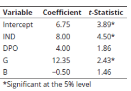
Practice Questions: Q5 Answer
Explanation: C is correct.
The t-statistic tests the null that industry P/Es are equal. The dummy variable is significant and positive, and the dummy variable is defined as being equal to one for biotechnology stocks, which means that biotechnology P/Es are statistically significantly larger than electric utility P/Es. Remember, however, this is only accurate if we hold the other independent variables in the model constant.
Practice Questions: Q6
Q6. Phil Ohlmer estimates a cross sectional regression in order to predict price to earnings ratios (P/E) with fundamental variables that are related to P/E, including dividend payout ratio (DPO), growth rate (G), and beta (B). In addition, all 50 stocks in the sample come from two industries, electric utilities or biotechnology. He defines the following dummy variable:
The results of his regression are shown in the following table.
Ohlmer is valuing a biotechnology stock with a dividend payout ratio of 0.00, a beta of 1.50, and an expected earnings growth rate of 0.14. The predicted P/E on the basis of the values of the explanatory variables for the company is closest to:
A. 7.7.
B. 15.7.
C. 17.2.
D. 11.3.
\begin{aligned}IND &=0 \text{ if the stock is in the electric utilities industry or}\\
&=1 \text{if the stock is in the biotechnology industry}\end{aligned}
Practice Questions: Q6 Answer
Explanation: B is correct.
Note that IND = 1 because the stock is in the biotech industry. Predicted P/E = 6.75 + (8.00 × 1) + (4.00 × 0.00) + (12.35 × 0.14) − (0.50 × 1.5) = 15.7.
Topic 5. The F-Test
- Purpose: Evaluates whether a full model is superior to competing partial models by testing if additional independent variables contribute meaningfully to explaining variation in Y
- Example: Compare a model with three independent variables (X₁, X₂, X₃) against a model with only one variable (X₁) to determine if X₂ and X₃ add explanatory power
- Hypotheses:
- F-Statistic Formula for Comparing Models:
- where
- residual sum of squares of the full model
- residual sum of squares of the partial model
- coefficient of determination of the full model
- coefficient of determination of the partial model
- q = # restrictions imposed on the full model to arrive at partial model
- #independent variables in the full model
- Decision Rule: F-test is always one-tailed; if calculated F-statistic > critical F-value [with q degrees of freedom in numerator and in denominator], the full model contributes meaningfully
H_0: \beta_2=\beta_3=0 \text { versus } H_A: \text { either } \beta_2 \neq 0 \text { or } \beta_3 \neq 0
\mathrm{F}=\frac{\left(\mathrm{RSS}_{\mathrm{P}}-\mathrm{RSS}_{\mathrm{F}}\right) / \mathrm{q}}{\mathrm{RSS}_{\mathrm{F}} /\left(\mathrm{n}-\mathrm{k}_{\mathrm{F}}-1\right)}=\frac{\left(\mathrm{R}_{\mathrm{F}}^2-\mathrm{R}_{\mathrm{P}}^2\right) / \mathrm{q}}{\left(1-\mathrm{R}_{\mathrm{F}}^2\right) /\left(\mathrm{n}-\mathrm{k}_{\mathrm{F}}-1\right)}
RSS_F =
RSS_P =
\mathrm{R}_{\mathrm{F}}^2=
\mathrm{R}_{\mathrm{F}}^2=
\mathrm{R}_{\mathrm{F}}^2=
(n-\mathrm{k}_{\mathrm{F}}-1)
\mathrm{k}_{\mathrm{F}}=
Topic 5. The F-Test
- Example 1: Evaluating Additional Variables in CAPM:
- Given: and q = # variables removed = 2,
- The F-test statistic is computed as:
- Critical F-value at 5% significance (df numerator = 2, df denominator = 60) = 3.15
- Conclusion: F = 2.21 < 3.15, fail to reject H₀; full model does not contribute meaningfully (β₂ = β₃ = 0)
- Generic F-Test for Overall Model Significance: Tests whether all variables are jointly insignificant:
- Example 2: Testing Overall Model Significance:
- Given: 46 monthly observations, 5 independent variables, TSS = 460, RSS = 170
- ESS = TSS - RSS = 460 - 170 = 290
- F = (290 / 5) / [170 / (46 - 5 - 1)] = 58 / 4.25 = 13.65
- Critical F-value (df = 5 and 40) at 5% significance = 2.45
- Conclusion: F = 13.65 > 2.45, reject H₀; at least one independent variable is significantly different from zero
\mathrm{RSS}_{\mathrm{F}}=6,650 ; \mathrm{RSS}_{\mathrm{P}}=7,140 ; \mathrm{n}=64 ; \mathrm{k}_{\mathrm{F}}=3;
F=\frac{(7,140-6,650) / 2}{6,650 /(64-3-1)}=2.21
F=\frac{E S S / k}{R S S / (n-k-1)}
H_0: \beta_1=\beta_2=\beta_3=\ldots .=\beta_k=0 \text { versus } H_A: \text {at least one } \beta_j \neq 0
QA 8. Regression with Multiple Explanatory Variables
By Prateek Yadav


