Book 2. Quantitative Analysis

FRM Part 1

QA 8. Regression with Multiple Explanatory Variables

Presented by: Sudhanshu

Module 1. Multiple Regression

Module 2. Measures of Fit In Linear Regression

Module 1. Multiple Regression

Topic 1. ⁠Relative Assumptions of Single and Multiple Regression

Topic 2. Interpreting Multiple Regression Coefficients

Topic 3. Interpreting Multiple Regression Results

Topic 1. Relative Assumptions of Single and Multiple Regression

General Form of Multiple Regression Model:

Regression or slope coefficients; sensitivity of Y to changes in (controlling for all other Xs).

$α$ : Value of Y when all $X_{s} = 0$ .
$ϵ$ : Random error or shock; unexplained component of Y.
Assumptions of Single Regression (modified for multiple Xs):
1. The expected value of the error term, conditional on the independent variables, is zero:
2. All (Xs and Y) observations are i.i.d.
3. The variance of X is positive (otherwise estimation of $β$ would not be possible).
4. The variance of the errors is constant (i.e., homoskedasticity).
5. There are no outliers observed in the data.
Additional Assumption for Multiple Regression: X variables are not perfectly correlated (i.e., they are not perfectly linearly dependent). Each X variable should have some variation not fully explained by other X variables.

Y=\alpha+\beta_1 X_1+\beta_2 X_2+\ldots+\beta_k X_k+\epsilon

\beta_j:

X_j

[E(\epsilon_i|X_{i's})=0].

Practice Questions: Q1

Q1. Which of the following is not an assumption of single regression

A. There are no outliers in the data.

B. The variance of the independent variables is greater than zero.

C. Independent variables are not perfectly correlated.

D. Residual variance are homoskedastic.

Practice Questions: Q1 Answer

Explanation: C is correct.

This is an assumption for multiple regression and not for single regression.

Topic 2. Interpreting Multiple Regression Coefficients

For a multiple regression, the interpretation of a slope coefficient is that it captures the change in the dependent variable for a one-unit change in that independent variable, holding the other independent variables constant.
As a result, these are sometimes called partial slope coefficients.
Ordinary Least Squares (OLS) Estimation Process (Stepwise):
- Step 1: Individual explanatory variables are regressed against other explanatory variables.
- Step 2: The dependent variable is regressed against all other explanatory variables (excluding the one whose coefficient is being estimated).
- Step 3: The residuals from Step 2 are regressed against the residuals from Step 1 to estimate the slope coefficient.
- This ensures the slope coefficient is calculated after controlling for variation in other independent variables.

Practice Questions: Q2

Q2. Multiple regression was used to explain stock returns using the following variables: Dependent variable: RET= annual stock returns (%)
Independent variables: MKT= market capitalization=market capitalization / $1.0 million.

IND= industry quartile ranking (IND = 4 is the highest ranking)

FORT= Fortune 500 firm, where {FORT=1 if the stock is that of a Fortune 500 firm, FORT=0 if not a Fortune 500 stock}
The regression results are presented in the following table.

Based on the results in the table, which of the following most accurately represents the regression equation?

A. 0.43 + 3.09(MKT) + 2.61(IND) + 1.70(FORT).

B. 0.681 + 0.021(MKT) + 0.04(IND) + 0.139(FORT).

C. 0.522 + 0.0460(MKT) + 0.7102(IND) + 0.9(FORT).

D. 1.21 + 0.015(MKT) + 0.2725(IND) + 0.5281(FORT).

Practice Questions: Q2 Answer

Explanation: C is correct.

The coefficients column contains the regression parameters.

Practice Questions: Q3

Q3. Multiple regression was used to explain stock returns using the following variables: Dependent variable: RET= annual stock returns (%)
Independent variables: MKT= market capitalization=market capitalization / $1.0 million.

IND= industry quartile ranking (IND = 4 is the highest ranking)

FORT= Fortune 500 firm, where {FORT=1 if the stock is that of a Fortune 500 firm, FORT=0 if not a Fortune 500 stock}
The regression results are presented in the following table.

The expected amount of the stock return attributable to it being a Fortune 500 stock is closest to:

A. 0.522.

B. 0.046.

C. 0.710.

D. 0.900.

Practice Questions: Q3 Answer

Explanation: D is correct.

The regression equation is 0.522 + 0.0460(MKT) + 0.7102(IND) + 0.9(FORT). The coefficient on FORT is the amount of the return attributable to the stock of a Fortune 500 firm.

Topic 3. Interpreting Multiple Regression Results

Scenario 1: Single Independent Variable
- Regression:
- Interpretation: If increases by 1 unit, Y is expected to increase by 4.5 units.
Scenario 2: Adding a Second Independent Variable
- Regression:
- Notice the coefficient for changed from 4.5 to 2.5. This is expected unless is uncorrelated with .
- Interpretation: If increases by 1 unit, Y is expected to increase by 2.5 units, holding constant.
- The intercept (1.0) is the e xpected value of Y when all Xs are zero.
Example: Three-Factor Model
1. Return when

1. Impact if $R_{z}$ declines by 1%: Change in $R_{P} = - (0.23 \times - 1) = + 0.23%$
2. Expected return when all factors are 0: Intercept $= 1.70%$

Y=2.0+4.5X_1

X_1

Y=1.0+2.5X_1+6.0X_2

X_1

X_2

X_1

X_2

R_{P,i}=1.70+1.03 R_{m,i}-0.23 R_{z,i}+0.32 R_{v,i}

R_m=8\%, R_z=2\%, R_v=3\%:E(R_P)=1.70+(1.03 \times 8)-(0.23 \times 2)+(0.32 \times 3)=10.44\%

Module 2. Measures of Fit in Linear Regression

Topic 1. Goodness-of-Fit mMeasures for Single and Multiple Regressions

Topic 2. Coefficient of Determination

Topic 3. Adjusted

Topic 4. Joint Hypothesis Tests and Confidence Intervals

Topic 5. The F-Test

R^2

Topic 1. Goodness-of-Fit Measures for Single and Multiple Regressions

Standard Error of the Regression (SER): Measures the uncertainty about the accuracy of predicted values of the dependent variable. A stronger relationship means data points are closer to the regression line (smaller errors).
OLS Estimation: Minimizes the sum of squared differences between predicted and actual values.
Decomposition of Total Variation:
- The regression model explains the variation in Y:
- Therefore:

Which means: $TSS = ESS + RSS$
- $TSS = Total Sum of Squares$ (total variation in Y)
- $ESS = Explained Sum of Squares$ (variation in Y explained by the model)
- $RSS = Residual Sum of Squares$ (unexplained variation in Y)

\sum(Y_i -\bar{Y})^2

Y_i-\bar{Y}=(\hat{Y}_i-\bar{Y})+(Y_i-\hat{Y}_i)

\sum(Y_i-\bar{Y})^2=\sum(\hat{Y}_i-\bar{Y})^2+\sum(Y_i-\hat{Y})^2

Topic 1. Goodness-of-Fit Measures for Single and Multiple Regressions

Topic 2. Coefficient of Determination

Definition: The coefficient of determination ( ) is the proportion of variation in Y that is explained by the regression model.
- $= ESS / TSS = % of variation explained by the regression model$
For multiple regression, is the square of the correlation between Y and the predicted value of Y.
Limitations of as a sole measure of explanatory power:
1. almost always increases as independent variables are added, even if their marginal contribution is not statistically significant. This can lead to overestimating the regression's explanatory power.
2. is not comparable across models with different dependent (Y) variables.
3. There are no clear predefined values of to indicate if a model is "good." Even low values can provide valuable insight for noisy variables (e.g., currency values)

R^2

Topic 3. Adjusted

To overcome the problem of overestimating the impact of additional variables, researchers recommend adjusting for the number of independent variables.
Formula for Adjusted
- $n = number of observations$
- $k = number of independent variables$
Key Characteristics of Adjusted :
- will always be less than or equal to .
- Adding a new independent variable will increase , but it may either increase or decrease . If the new variable has only a small effect on , may decrease.
- may be less than zero if is low enough.

R^2

R^2 (R_a^2):

R_a^2=1-\left[\left(\frac{n-1}{n-k-1}\right)\times (1-R^2)\right]

R^2

R_a^2

R^2

R_a^2

R^2

R_a^2

R^2

Practice Questions: Q4

Q4. When interpreting the and adjusted measures for a multiple regression, which of the following statements incorrectly reflects a pitfall that could lead to invalid conclusions?

A. The measure does not provide evidence that the most or least appropriate independent variables have been selected.

B. If the is high, we have to assume that we have found all relevant independent variables.

C. If adding an additional independent variable to the regression improves the , this variable is not necessarily statistically significant.

D. The measure may be spurious, meaning that the independent variables may show a high ; however, they are not the exact cause of the movement in the dependent variable.

R^2

Practice Questions: Q4 Answer

Explanation: B is correct.

If the is high, we cannot assume that we have found all relevant independent variables. Omitted variables may still exist, which would improve the regression results further.

R^2

Topic 4. Joint Hypothesis Tests and Confidence Intervals

The magnitude of coefficients does not indicate the importance of independent variables. Hypothesis testing is needed to determine if variables significantly contribute to explaining the dependent variable.
t-statistic for Individual Coefficients:

Degrees of freedom for multiple regression: $(n - k - 1)$
Testing Statistical Significance ( versus ):
- Example: Test significance of PR at 10% level, $n = 46$ , critical t-value = 1.68.
  - PR coefficient = 0.25, Standard Error = 0.032
  - Since $7.8 > 1.68$ , reject $H_{0}$ . PR is statistically significantly different from zero.

Confidence Interval for a Regression Coefficient:

t=\frac{b_j-B_j}{s_{b_j}}=\frac{\text { estimated regression coefficient-hypothesized value }}{\text { coefficient standard error of } b_j}

H_0:b_j=0

H_A:b_j \neq 0

t=0.25/0.032=7.8

b_j \pm (t_c \times s_{b_{j}})

Practice Questions: Q5

Q5. Phil Ohlmer estimates a cross sectional regression in order to predict price to earnings ratios (P/E) with fundamental variables that are related to P/E, including dividend payout ratio (DPO), growth rate (G), and beta (B). In addition, all 50 stocks in the sample come from two industries, electric utilities or biotechnology. He defines the following dummy variable:

The results of his regression are shown in the following table.

Based on these results, it would be most appropriate to conclude that:
A. biotechnology industry P/Es are statistically significantly larger than electric
utilities industry P/Es.
B. electric utilities P/Es are statistically significantly larger than biotechnology
industry P/Es, holding DPO, G, and B constant.
C. biotechnology industry P/Es are statistically significantly larger than electric
utilities industry P/Es, holding DPO, G, and B constant.
D. the dummy variable does not display statistical significance.

\begin{aligned}IND &=0 \text{ if the stock is in the electric utilities industry or}\\ &=1 \text{if the stock is in the biotechnology industry}\end{aligned}

Practice Questions: Q5 Answer

Explanation: C is correct.

The t-statistic tests the null that industry P/Es are equal. The dummy variable is significant and positive, and the dummy variable is defined as being equal to one for biotechnology stocks, which means that biotechnology P/Es are statistically significantly larger than electric utility P/Es. Remember, however, this is only accurate if we hold the other independent variables in the model constant.

Practice Questions: Q6

Q6. Phil Ohlmer estimates a cross sectional regression in order to predict price to earnings ratios (P/E) with fundamental variables that are related to P/E, including dividend payout ratio (DPO), growth rate (G), and beta (B). In addition, all 50 stocks in the sample come from two industries, electric utilities or biotechnology. He defines the following dummy variable:

The results of his regression are shown in the following table.

Ohlmer is valuing a biotechnology stock with a dividend payout ratio of 0.00, a beta of 1.50, and an expected earnings growth rate of 0.14. The predicted P/E on the basis of the values of the explanatory variables for the company is closest to:

A. 7.7.

B. 15.7.

C. 17.2.

D. 11.3.

\begin{aligned}IND &=0 \text{ if the stock is in the electric utilities industry or}\\ &=1 \text{if the stock is in the biotechnology industry}\end{aligned}

Practice Questions: Q6 Answer

Explanation: B is correct.

Note that IND = 1 because the stock is in the biotech industry. Predicted P/E = 6.75 + (8.00 × 1) + (4.00 × 0.00) + (12.35 × 0.14) − (0.50 × 1.5) = 15.7.

Topic 5. The F-test

Purpose: The F-test is useful to evaluate a model against other competing partial models, especially when testing complex hypotheses involving the impact of more than one variable (where the univariate t-test is not applicable).
Hypothesis for comparing models (e.g., full vs. partial):
- $H_{0} : β_{2} = β_{3} = 0$ (additional variables do not contribute meaningfully)
- $H_{A} : either$ (at least one additional variable contributes)
F-statistic for multiple regression coefficients (one-tailed test):

$RS S_{F}$ : Residual sum of squares of the full model
$RS S_{P}$ : Residual sum of squares of the partial model
: Coefficient of determination of the full model
: Coefficient of determination of the partial model
$q$ : Number of restrictions imposed (variables removed)
$n$ : Number of observations
$k_{F}$ : Number of independent variables in the full model
Decision Rule: If calculated F-statistic $>$ critical F-value (with q and $(n - k_{F} - 1)$ degrees of freedom), reject $H_{0}$ .

\beta_2 \neq 0 \text{ or }\beta_3 \neq 0

F=\frac{(RSS_P -RSS_F)/q}{RSS_F/ (n-k_F -1)}=\frac{(R_F^2 -R_P^2)/q}{(-R_F^2)/(n-k_F-1)}

R_F^2

R_P^2

QA 8. Regression with Multiple Explanatory Variables

By Prateek Yadav

QA 8. Regression with Multiple Explanatory Variables

Book 2. Quantitative Analysis

FRM Part 1

QA 8. Regression with Multiple Explanatory Variables

Presented by: Sudhanshu

Module 1. Multiple Regression

Module 2. Measures of Fit In Linear Regression

Module 1. Multiple Regression

Topic 1. Relative Assumptions of Single and Multiple Regression

Practice Questions: Q1

Practice Questions: Q1 Answer

Topic 2. Interpreting Multiple Regression Coefficients

Practice Questions: Q2

Practice Questions: Q2 Answer

Practice Questions: Q3

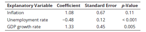
Practice Questions: Q3 Answer

Topic 3. Interpreting Multiple Regression Results

Module 2. Measures of Fit in Linear Regression

Topic 1. Goodness-of-Fit Measures for Single and Multiple Regressions

Topic 1. Goodness-of-Fit Measures for Single and Multiple Regressions

Topic 2. Coefficient of Determination

Topic 3. Adjusted

Practice Questions: Q4

Practice Questions: Q4 Answer

Topic 4. Joint Hypothesis Tests and Confidence Intervals

Practice Questions: Q5

Practice Questions: Q5 Answer

Practice Questions: Q6

Practice Questions: Q6 Answer

Topic 5. The F-test

QA 8. Regression with Multiple Explanatory Variables

More from Prateek Yadav