Book 2. Quantitative Analysis
FRM Part 1
QA 6. Hypothesis Testing
Presented by: Sudhanshu
Module 1. Hypothesis Testing Basics
Module 2. Hypothesis Testing Results
Module 1. Hypothesis Testing Basics

Topic 1. Basics of Hypothesis Testing
Topic 2. Null Hypothesis and Alternative Hypothesis
Topic 3. Choice of the Null and Alternative Hypotheses
Topic 4. Two-Tailed Hypotheses Testing
Topic 5. One-Tailed Hypotheses Testing
Topic 6. Type I and Type II Errors
Topic 7. Type I and II Errors in Hypothesis Testing
Topic 8. Relation Between Confidence Intervals and Hypothesis Tests
Topic 9. Statistical Significance vs. Practical Significance
Topic 1. Basics of Hypothesis Testing
- Definition: A statistical method used to evaluate assumptions about a population using sample data.
- Main Purpose: Assess whether observed data supports a specific claim or belief.
-
6 Key Elements:
- Null Hypothesis (H₀): Statement assumed to be true initially (e.g., µ = µ₀).
- Alternative Hypothesis (Hₐ): Contradicts H₀ and represents what we aim to support.
-
Test Statistic: Measures deviation of sample statistic from hypothesized value.
-
Significance Level (α): Probability of rejecting true H₀ (commonly 0.01, 0.05, 0.10).
-
Critical Value: Based on α, determines rejection regions.
-
Decision Rule: "Reject H₀ if test statistic > critical value".
- Applications: Portfolio return testing, risk factor analysis, economic indicators.
Topic 2. Null Hypothesis and Alternative Hypothesis
-
Null Hypothesis ( ):
- Specifies a value assumed to be true (e.g., H₀: µ = 5%).
- Always includes the equality (e.g., ≤, ≥, =).
-
Alternative Hypothesis ( ):
- Reflects the outcome we suspect or want to prove.
- Does not include the equality.
-
Example:
- Claim: Mean return > 0
- Why We Reject H₀ Instead of Proving Hₐ: Statistics cannot confirm truth; only provide evidence against assumptions.
H_0
H_A
H_0: \mu \leq 0
H_A: \mu>0
Practice Questions: Q1
Q1.Austin Roberts believes the mean price of houses in the area is greater than $145,000. A random sample of 36 houses in the area has a mean price of $149,750. The population standard deviation is $24,000, and Roberts wants to conduct a hypothesis test at a 1% level of significance. The appropriate alternative hypothesis is:
A.
B.
C.
D.
H_A: \mu>\$ 145,000 .
H_A: \mu \geq \$ 145,000 .
\mathrm{H}_A: \mu \pm \$ 145,000 .
\mathrm{H}_A: \mu>\$ 145,000 .
Practice Questions: Q1 Answer
Explanation: D is correct.
\mathrm{H}_{\mathrm{A}}: \mu>\$ 145,000
Topic 3. Choice of the Null and Alternative Hypotheses
-
Choose hypotheses that allow a clear decision rule:
- If you're testing effectiveness, set H₀ as "no effect."
- Example: Testing fund manager skill: H₀: α = 0 (no skill), : α ≠ 0
-
Align with research goals:
- Testing for improvement → H₀: new method ≤ old method
- Testing for difference → H₀: µ₁ = µ₂
-
Hypothesis testing involves two statistics: the test statistic calculated from the sample data and the critical value of the test statistic.
-
A test statistic is calculated by comparing the point estimate of the population parameter with the hypothesized value of the parameter (i.e., the value specified in the null hypothesis).
-
The test statistic is the difference between the sample statistic and the hypothesized value, scaled by the standard error of the sample statistic:
-
The standard error of the sample statistic is the adjusted standard deviation of the sample.
-
-
-
H_A
\text { test statistic }=\frac{\text { sample statistic }- \text { hypothesized value }}{\text { standard error of the sample statistic }}
\sigma_{\bar{x}}=\frac{\sigma}{\sqrt{n}}; \text{ when the population standard deviation, σ, is known }
s_{\bar{x}}=\frac{s}{\sqrt{n}}; \text{ when the population standard deviation, σ, is not known }
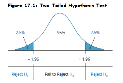
Topic 4. Two-Tailed Hypotheses Testing
-
A two-sided test is referred to as a two-tailed test.
- Used When: Interested in detecting difference in either direction (greater or smaller).
-
A two-tailed test for the population mean may be structured as:
- Critical Values: A two-tailed test uses two critical values (or rejection points).
-
Decision Rule: The general decision rule for a two-tailed test is:
-
Example: Consider a z-test at a 5% level of significance, α = 0.05 (z-value=±1.96)
- Reject H₀ if test statistic > 1.96 or < –1.96
- Example: Mean return = 0, if test statistic = 2.5 → Reject H₀.
H_0: \mu=\mu_0 \text{ Vs } H_A: \mu \neq \mu_0
\begin{aligned}
\text { Reject } \mathrm{H}_0 & \text { if: test statistic > upper critical value or } \\
\text { Reject } \mathrm{H}_0 &\text { if: test statistic < lower critical value}
\end{aligned}
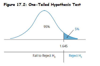
Topic 5. One-Tailed Hypotheses Testing
-
A one-sided test is referred to as a one-tailed test. In practice, most hypothesis tests are constructed as two-tailed tests.
- Used When: Only deviation in one direction matters.
- Upper-Tailed Test:
- Lower-Tailed Test:
- Critical Values: A one-tailed test uses one critical value (or rejection point).
-
Decision Rule: The general decision rule for a one-tailed test is:
- Reject H₀ if z > critical value (upper-tailed test)
- Reject H₀ if z < critical value (lower-tailed test)
- Example: Consider a z-test at a 5% level of significance, α = 0.05 (z-value=1.645)
- Mean return = 0. If z = 2.33 > 1.645 (test-statistic) → Reject H₀.
H_0: \mu \leq \mu_0 \text{ Vs } H_A: \mu>\mu_0
H_0: \mu \geq \mu_0 \text{ Vs } H_A: \mu<\mu_0
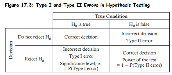
Topic 6. Type I and Type II Errors
-
Type I Error (α):
- Rejecting H₀ when H₀ is true.
- The significance level is the probability of making a Type I error
-
Type II Error (β):
- Failing to reject H₀ when H₀ is false.
-
Power of the Test= 1 – β
- It indicates probability of detecting a true effect.
-
Trade-Off:
- Lower α increases β.
- Increasing sample size reduces both α and β.
Topic 7. Type I and II Errors in Hypothesis Testing
-
Error Implications:
- Type I: False alarm (e.g., wrongly detect alpha > 0).
- Type II: Missed opportunity (e.g., miss real alpha).
-
Graphical Representation:
- Overlapping null and alternative distributions.
-
Sample Size Impact:
- Larger n → smaller standard error → more power.
-
α and β Relationship:
- Decreasing α increases β (unless n increases).
Practice Questions: Q2
Q2. Which of the following statements about hypothesis testing is most accurate?
A. The power of a test is one minus the probability of a Type I error.
B. The probability of a Type I error is equal to the significance level of the test.
C. To test the claim that X is greater than zero, the null hypothesis would be : X > 0.
D. If you can disprove the null hypothesis, then you have proven the alternative hypothesis.
H_0
Practice Questions: Q2 Answer
Explanation: B is correct.
The probability of getting a test statistic outside the critical value(s) when the null is true is the level of significance and is the probability of a Type I error. The power of a test is one minus the probability of a Type II error. Hypothesis testing does not prove a hypothesis; we either reject the null or fail to reject it. The appropriate null would be X ≤ 0 with X > 0 as the alternative hypothesis.
Topic 8. Relation Between Confidence Intervals and Hypothesis Tests
-
Confidence Interval (CI): Range of values where the true population parameter lies with a specified probability.
-
A confidence interval for a two-tailed test is determined as:
-
-
It can also be written as:
-
Confidence intervals can also be provided for one-tailed tests as either:
-
Upper tail:
- Lower tail:
-
- Link to Hypothesis Test: If H₀ value lies outside CI → Reject H₀.
-
Two-Tailed Test Example:
- CI = [0.03%, 0.17%]; H₀: µ = 0 → 0 is not in interval → Reject H₀.
\bar{x} \pm z_{\alpha / 2} \times \frac{\sigma}{\sqrt{n}}
\left\{\left[\begin{array}{c}
\text { sample } \\
\text { statistic }
\end{array}-\binom{\text { critical }}{\text { value }}\binom{\text { standard }}{\text { error }}\right] \leq \begin{array}{c}
\text { population } \\
\text { parameter }
\end{array} \leq\left[\begin{array}{c}
\text { sample } \\
\text { statistic }
\end{array}+\binom{\text { critical }}{\text { value }}\binom{\text { standard }}{\text { error }}\right]\right\}
\left\{\left[\begin{array}{l}
\text { sample } \\
\text { statistic }
\end{array}-\binom{\text { critical }}{\text { value }}\binom{\text { standard }}{\text { error }}\right] \leq \begin{array}{l}
\text { population } \\
\text { parameter }
\end{array} \leq \infty\right\}
\left\{-\infty \leq \begin{array}{l}
\text { population } \\
\text { parameter }
\end{array} \leq\left[\begin{array}{c}
\text { sample } \\
\text { statistic }
\end{array}+\binom{\text { critical }}{\text { value }}\binom{\text { standard }}{\text { error }}\right]\right\}
Topic 9. Statistical Significance vs. Practical Significance
- Statistical Significance:
- result unlikely under H₀.
-
Practical Significance:
- Is the effect meaningful in context?
-
Real-World Factors:
- Transaction costs, risk, taxes can erode “statistically significant” returns.
-
Large Samples:
- Even tiny effects may become statistically significant.
p<\alpha \rightarrow
Module 2. Hypothesis Testing Results
Topic 1. The p-Value
Topic 2. The t-Test
Topic 3. The z-Test
Topic 4. Testing the Equality of Means
Topic 5. Multiple Hypothesis Testing
Topic 1. The p-Value
- Definition: Probability of obtaining a test statistic that would lead to a rejection of the null hypothesis, assuming H₀ is true.
- Interpretation: Smallest level of significance for which the null hypothesis can be rejected.
- One-tailed tests: The p-value represents the probability above the computed test statistic for upper tail tests, or below the computed test statistic for lower tail tests.
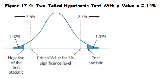
- Two-tailed tests: The p-value is calculated as the combined probability above the positive value of the test statistic plus the probability below the negative value of the test statistic.
- Test setup: Two-tailed hypothesis test at 95% significance level with test statistic of 2.3, which exceeds the critical value of 1.96. Probability above 2.3 is 1.07% from z-table; for two-tailed test, p-value = 2 × 1.07% = 2.14%.
- Decision rule: Reject null hypothesis at 3%, 4%, or 5% significance levels, but fail to reject at 2% or 1% significance levels.
- Many researchers report p-values without pre-selecting significance levels, allowing readers to assess the strength of evidence independently.
Practice Questions: Q2
Q2. Austin Roberts believes the mean price of houses in the area is greater than $145,000. A random sample of 36 houses in the area has a mean price of $149,750. The population standard deviation is $24,000, and Roberts wants to conduct a hypothesis test at a 1% level of significance. The value of the calculated test statistic is closest to:
A. z = 0.67.
B. z = 1.19.
C. z = 4.00.
D. z = 8.13.
Practice Questions: Q2 Answer
Explanation: B is correct.
z=\frac{149,750-145,000}{24,000 / \sqrt{36}}=1.1875
Topic 2. The t-Test
-
Employs a test statistic that is distributed according to a t-distribution.
-
Used when population variance is unknown and either of the following
conditions exist:
- The sample is large (n ≥ 30).
-
The sample is small (n < 30), but the distribution of the population is normal or approximately normal.
-
If the sample is small and the distribution is non-normal, we have no reliable statistical test.
-
For hypothesis tests of a population mean, a t-statistic with n − 1 degrees of freedom is computed as:
-
Example:
- Sample mean = 8, s = 2, n = 25, µ₀ = 7
- t = 2.5, df = 24 → compare with t-critical
-
In the real world, the underlying variance of the population is rarely known, so the t-test enjoys widespread application.
t=\frac{\bar{x}-\mu_0}{s / \sqrt{n}}, \quad \mathrm{df}=n-1
Topic 3. The z-Test
-
Appropriate hypothesis test of the population mean when the population is normally distributed with known variance.
-
The z-statistic for a hypothesis test for a population mean is computed as follows:
-
Example:
-
Sample mean = 2.49, σ = 0.021, n = 49
-
H₀: µ = 2.5 → z = –3.33 → Reject H₀
-
-
Critical z-values for the most common levels of significance are given below (Memorize these).
-
When the sample size is large and the population variance is unknown, the z-statistic is:
z=\frac{\bar{x}-\mu_0}{s / \sqrt{n}}

z=\frac{\bar{x}-\mu_0}{\sigma / \sqrt{n}}
Practice Questions: Q3
Q3. Austin Roberts believes the mean price of houses in the area is greater than $145,000. A random sample of 36 houses in the area has a mean price of $149,750.
The population standard deviation is $24,000, and Roberts wants to conduct a hypothesis test at a 1% level of significance. The value of the calculated test statistic is closest to:
A. z = 0.67.
B. z = 1.19.
C. z = 4.00.
D. z = 8.13.
Practice Questions: Q3 Answer
Explanation: B is correct.
z=\frac{149,750-145,000}{24,000 / \sqrt{36}}=1.1875
Topic 4. Testing the Equality of Means
- Two-population mean comparison: Finance applications frequently require testing whether the means of two populations are equal, which is equivalent to testing if their difference equals zero.
- Statistical assumptions: The test assumes two series (X and Y) are each independent and identically distributed (i.i.d.) with a defined covariance Cov(X,Y).
-
Test statistic framework: When these assumptions are met, a specific test statistic formula is used to evaluate the hypothesis about the difference between population means.
-
- Distribution property: The test statistic follows a standard normal distribution when the null hypothesis is true.
- Hypothesis formulation: Null hypothesis states the difference between means equals zero; alternative hypothesis states it does not equal zero.
- Decision process: Compare the calculated test statistic to the critical value based on chosen test size to either reject or fail to reject the null hypothesis.
T=\frac{\bar{X}-\bar{Y}}{\sqrt{\frac{s_X^2+s_Y^2-2 \operatorname{Cov}(X, Y)}{n}}}
Topic 5. Multiple Hypothesis Testing
- Multiple testing definition: Testing multiple different hypotheses on the same dataset, such as comparing 10 active trading strategies against a buy-and-hold strategy.
- Rejection probability issue: Repeatedly testing different strategies against the same null hypothesis makes it highly likely that at least one will be incorrectly rejected by chance.
- Alpha inflation problem: The stated alpha (probability of Type I error) is only accurate for single hypothesis tests; actual alpha increases with each additional test performed.
- Type I error consequence: As the actual alpha grows larger through multiple testing, the probability of incorrectly rejecting a true null hypothesis (Type I error) increases substantially.
Practice Questions: Q4
Q4. The most likely bias to result from testing multiple hypotheses on a single data set is that the value of:
A. a Type I error will increase.
B. a Type II error will increase.
C. the critical value will increase.
D. the test statistic will increase.
Practice Questions: Q4 Answer
Explanation: A is correct.
With multiple testing, the alpha (the probability of incorrectly rejecting a true null) is only accurate for one single hypothesis test. As we test more and more strategies, the actual alpha of this repeated testing grows larger, and as alpha grows larger, the probability of a Type I error increases.
QA 6. Hypothesis Testing
By Prateek Yadav


