Book 2. Quantitative Analysis
FRM Part 1
QA 3. Common Univariate Random Variables
Presented by: Sudhanshu
Module 1. Uniform, Bernoulli, Binomial and Poisson Distributions
Module 2. Normal and Lognormal Distributions
Module 3. Student's T, Chi-Squared, F- and Other Distributions
Module 1. Uniform, Bernoulli, Binomial and Poisson Distributions

Topic 1. The Uniform Distribution
Topic 2. The Bernoulli Distribution
Topic 3. The Binomial Distribution
Topic 4. The Poisson Distribution
Topic 1. The Uniform Distribution
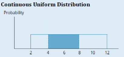
- Definition: The continuous uniform distribution is defined over a range spanning between a lower limit (a) and an upper limit (b), which act as its parameters. Outcomes occur only between a and b.
-
Properties:
- The probability of X outside the boundaries (a and b) is zero.
- The probability of outcomes between any two points and within the range is given by:
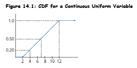
- The cumulative distribution function (CDF) is linear over the variable's range.
- The probability density function (PDF) is expressed as: for a ≤ x ≤ b, otherwise f(x) = 0.
- Parameters: Lower limit (a) and upper limit (b).
- Mean:
- Variance:
- Example: For X uniformly distributed between 2 and 12, the probability that X will be between 4 and 8 is (8-4)/(12-2) = 4/10 = 40%.
x_1
x_2
P(x_1 ≤ X ≤ x_2) = \frac{(x_2 - x_1)}{(b - a)}
f(x)=\frac{1}{b-a}
E(x)=\frac{(a+b)}{2}
Var(x) =\frac{ (b - a)^2} { 12}
Topic 1. The Uniform Distribution
- The PDF and CDF of a uniform distribution are shown in below figures
Practice Questions: Q3
Q3. What is the probability of an outcome being between 15 and 25 for a random variable that follows a continuous uniform distribution within the range of 12 to 28?
A. 0.509.
B. 0.625.
C. 1.000.
D. 1.600.
Practice Questions: Q3 Answer
Explanation: B is correct.
Since a = 12 and b = 28:
P(15 \leq X \leq 25)=\frac{(25-15)}{(28-12)}=\frac{10}{16}=0.625
Topic 2. The Bernoulli Distribution
- Definition: A Bernoulli random variable has only two possible outcomes, typically defined as success (denoted with value 1) or failure (denoted with value 0).
- Common Occurrences: Used for assessing the probability of binary outcomes, such as the probability that a firm will default on its debt.
-
Properties:
- Probability of success is p, and probability of failure is 1 - p.
- The probability mass function (PMF) is , yielding P(x=1) = p and P(x=0) = 1-p.
- Parameters: p (probability of success).
- Mean:
- Variance: Var(X) = p(1-p). Maximum variance is at p = 0.5.
-
CDF:
- F(x) = 0 for x < 0
- F(x) = 1 - p for 0 ≤ x < 1
- F(x) = 1 for x ≥ 1
f(x) = p^x (1-p)^{(1-x)}
\mu_x=p
Topic 3. The Binomial Distribution
- Definition: A binomial random variable represents the number of successes in a given number of Bernoulli trials, where each trial has an outcome of either success or failure.
-
Properties:
- The probability of success (p) is constant for each trial.
- Trials are independent.
- The binomial probability function defines the probability of exactly x successes in n trials.
- Formula (Probability of exactly x successes in n trials):
- Parameters: n (number of trials) and p (probability of success on each trial).
- Expected Value: E(X) = np
- Variance: Var(X) = np(1-p)
- Common Occurrences: Extensively used in the investment world where outcomes are seen as successes or failures (e.g., security price going up or down). Often used to create models for asset valuation.
P(x) = P(X = x) = \left[\frac{n!} { ((n - x)! x!)}\right]* p^x *(1 - p)^{(n-x)}
Practice Questions: Q2
Q2. A recent study indicated that 60% of all businesses have a web page. Assuming a binomial probability distribution, what is the probability that exactly four businesses will have a web page in a random sample of six businesses?
A. 0.138.
B. 0.276.
C. 0.311.
D. 0.324.
Practice Questions: Q2 Answer
Explanation: C is correct.
Success = having a web page:
\left[\frac{6!}{4! (6-4)!}\right](0.6)^4(0.4)^{6-4}=15(0.1296)(0.16)=0.311
Topic 4. The Poisson Distribution
- Definition: A discrete probability distribution.
- Common Occurrences: Models the number of successes per unit. Examples include the number of defects per batch in a production process or the number of 911 calls per hour.
-
Properties:
- Both its mean and variance are equal to the parameter, λ (lambda).
- Formula (Probability of obtaining X successes, given λ successes are expected):
- Parameters: λ (average or expected number of successes per unit).
- Mean: λ
- Variance: λ
P(X = x) = \frac{(λ^x * e^-λ)}{ x!}
Practice Questions: Q1
Q1. If 5% of the cars coming off the assembly line have some defect in them, what is the probability that out of three cars chosen at random, exactly one car will be defective? Assume that the number of defective cars has a Poisson distribution.
A. 0.129.
B. 0.135.
C. 0.151.
D. 0.174.
Practice Questions: Q1 Answer
Explanation: A is correct.
The probability of a defective car (p) is 0.05; hence, the probability of a nondefective car (q) = 1 − 0.05 = 0.95. Assuming a Poisson distribution:
λ = np = (3)(0.05) = 0.15
Then,
P(X=1)=\frac{\lambda^x e^{-\lambda}}{x!}=\frac{(0.15)^1 e^{-0.15}}{1!}=0.129106
Module 2. Normal and Lognormal Distributions
Topic 1. The Normal Distribution: Basics
Topic 2. Confidence Intervals for Normal Distribution
Topic 3. The Standard Normal Distribution
Topic 4. Calculating Probabilities Using z-Values
Topic 5. The Lognormal Distribution
Topic 1. The Normal Distribution: Basics
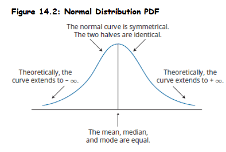
- Definition: A symmetrical, bell-shaped continuous probability distribution.
- Importance: Many random variables relevant to finance and other professional disciplines follow a normal distribution. Plays a central role in portfolio theory.
- PDF:
-
Key Properties:
- Completely described by its mean (μ) and variance , denoted as
- Skewness = 0 => symmetric about mean => P(X ≤ μ) = P(μ ≤ X) = 0.5 & mean = median = mode.
- Kurtosis = 3: This measures the spread with emphasis on the tails. Excess kurtosis is measured relative to 3.
- A linear combination of normally distributed independent RVs is also normally distributed.
- Probabilities of outcomes further from the mean get smaller but do not reach 0 (tails extend infinitely).
(\sigma^2)
X \sim N(\mu, \sigma^2).
f(x)=\frac{1}{\sigma \sqrt{2 \pi}} e^{-\frac{1}{2}\left(\frac{x-\mu}{\sigma}\right)^2}
Topic 2. Confidence Intervals for Normal Distribution
-
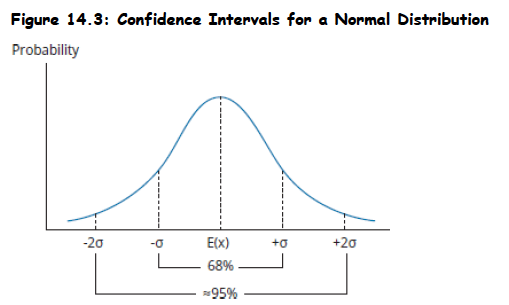
A confidence interval defines a range of values around an expected outcome where we anticipate the actual result will fall a specified percentage of the time (e.g., 95% confidence interval means we expect the true value to be within that range 95% of the time).
-
For normal distributions, confidence intervals are constructed using the expected value (mean) and standard deviation, with 68% of outcomes falling within one standard deviation and approximately 95% within two standard deviations of the mean.
-
In real-world applications, we estimate the true mean and standard deviation using sample statistics (X̄ and s) since the actual population parameters are typically unknown.
-
Common confidence intervals use specific multipliers of the standard deviation: 90% confidence uses ±1.65s, 95% confidence uses ±1.96s, and 99% confidence uses ±2.58s around the sample mean.
-
The wider the confidence interval (higher confidence percentage), the more certain we can be that the true population parameter falls within that range, but at the cost of precision in our estimate.
Topic 3. The Standard Normal Distribution
- A standard normal distribution (z-distribution) is a normal distribution with a mean of 0 and standard deviation of 1, denoted as N∼(0,1).
- The z-value represents how many standard deviations a specific observation is away from the population mean.
- Standardization is the process of converting any observed value from a normal distribution into its corresponding z-value.
- This conversion allows comparison of observations from different normal distributions on a common scale.
- The standardization process uses a specific formula to transform the original observation into a z-score.
\mathrm{z}=\frac{\text { observation }- \text { population mean }}{\text { standard deviation }}=\frac{\mathrm{x}-\mu}{\sigma}
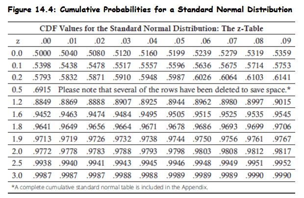
Topic 4. Calculating Probabilities Using z-Values
-
Z-table purpose: The z-table contains cumulative density function values for a standard normal distribution, showing probabilities P(Z < z) for standardized values.
-
Table structure: The first column lists z-values with one decimal place, while subsequent columns provide probabilities for z-values extended to two decimal places.
-
Positive values only: The table typically shows only positive z-values, which is sufficient due to the symmetric property of the normal distribution.
-
Symmetry property: For negative z-values, the relationship F(−Z) = 1 − F(Z) allows calculation of probabilities using the positive z-value probabilities.
-
Practical application: These standardized z-values and their corresponding probabilities enable determination of probabilities for any normal distribution after standardization.
Practice Questions: Q4
Q4. The probability that a normal random variable will be more than two standard deviations above its mean is:
A. 0.0217.
B. 0.0228.
C. 0.4772.
D. 0.9772.
Practice Questions: Q4 Answer
Explanation: B is correct.
1-F(2)=1-0.9772=0.0228
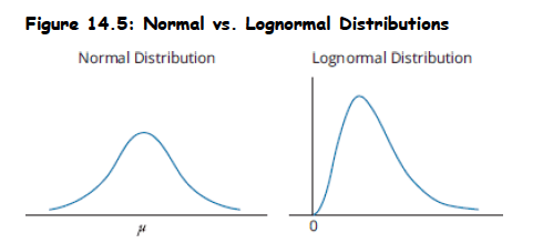
Topic 5. The Lognormal Distribution
- Definition: Generated by the function , where x is normally distributed. The natural logarithms of lognormally distributed random variables are normally distributed.
-
Pdf of lognormal distribution:
-
-
Key Properties:
- Skewed to the right.
- Bounded from below by zero, making it useful for modeling asset prices that cannot take negative values. This avoids the problem of negative asset prices that a normal distribution of returns might imply.
- Common Occurrences: Useful for modeling asset prices and price relatives (end-of-period price divided by beginning price)
e^x
f(x)=\frac{1}{x \sigma \sqrt{2 \pi}} e^{-\frac{1}{2}\left(\frac{\ln x-\mu}{\sigma}\right)^2}
Practice Questions: Q5
Q5. Which of the following random variables is least likely to be modeled appropriately by a lognormal distribution?
A. The size of silver particles in a photographic solution.
B. The number of hours a housefly will live.
C. The return on a financial security.
D. The weight of a meteor entering the earth’s atmosphere.
Practice Questions: Q5 Answer
Explanation: C is correct.
A lognormally distributed random variable cannot take on values less than zero. The return on a financial security can be negative. The other choices refer to variables that cannot be less than zero.
Module 3. Student's T, Chi-Squared, F-and Other Distributions
Topic 1. Student's t-distribution
Topic 2. The Chi-squared distribution
Topic 3. The F-Distribution
Topic 4. The Exponential Distribution
Topic 5. The Beta Distribution
Topic 6. Mixture Distributions
Topic 1. Student's t-distribution
- Definition: Similar to a normal distribution but has "fatter tails" (a greater proportion of outcomes in the tails).
-
When to Use:
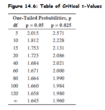
- Appropriate for constructing confidence intervals based on small samples (n < 30) from a population with unknown variance and a normal (or approximately normal) distribution.
- Can also be used with larger samples when population variance is unknown, and the Central Limit Theorem ensures an approximately normal sampling distribution.
-
Key Properties:
- Symmetrical.
- Defined by a single parameter: degrees of freedom (df), which is equal to the number of sample observations minus 1 (n - 1) for sample means.
- Has a greater probability in the tails (fatter tails) than the normal distribution.
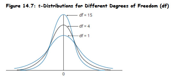
- As the degrees of freedom (sample size) increase, the shape of the t-distribution more closely approaches a standard normal distribution.
- Confidence intervals for a t-distribution must be wider than those for a normal distribution at a given confidence level.
Topic 1. Student's t-distribution
- The t-distribution's shape varies with degrees of freedom, becoming more similar to the normal distribution as degrees of freedom increase.
- Higher degrees of freedom result in more observations concentrated near the center and fewer observations in the distribution's tails.
- As degrees of freedom increase, the tails of the t-distribution become thinner, approaching the shape of a normal distribution.
- T-distribution confidence intervals are wider than normal distribution intervals at the same confidence level due to the distribution's thicker tails.
Practice Questions: Q6
Q6. The t-distribution is the appropriate distribution to use when constructing confidence intervals based on:
A. large samples from populations with known variance that are nonnormal.
B. large samples from populations with known variance that are at least approximately normal.
C. small samples from populations with known variance that are at least approximately normal.
D. small samples from populations with unknown variance that are at least approximately normal.
Practice Questions: Q6 Answer
Explanation: D is correct.
The t-distribution is the appropriate distribution to use when constructing conidence intervals based on small samples from populations with unknown variance that are either normal or approximately normal.
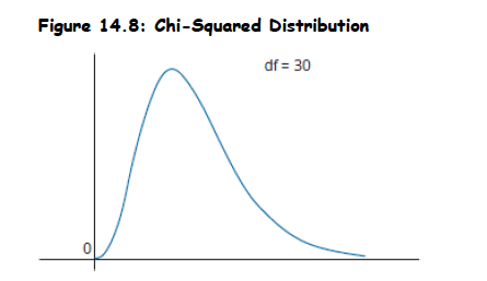
Topic 2. The Chi-Squared Distribution
- When to Use: Often used for hypothesis tests concerning population parameters and models of random variables that are always positive.
- Properties: An asymmetrical distribution bounded below by zero. Approaches the normal distribution in shape as the degrees of freedom increase.
-
The chi-squared test statistic, , with n − 1 degrees of freedom, is computed as:
-
- The chi-squared test compares the test statistic to a critical chi-squared value at a given level of significance to determine whether to reject or fail to reject a null hypothesis.
\chi^2
\begin{aligned} \chi_{n-1}^2=\frac{(n-1) s^2}{\sigma_0^2}; n&=\text{ sample size }, s^2 = \text{sample variance and } \\ \quad \sigma_0^2&=\text{hypothesized value for the population variance} \end{aligned}
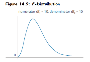
Topic 3. The F-Distribution
- Used to test hypotheses concerning the equality of the variances of two populations.
- Requires that the populations from which samples are drawn are normally distributed and samples are independent.
- Test Statistic: The F-statistic is computed as the ratio of the sample variances:
-
Properties:
- A right-skewed distribution truncated at zero on the left-hand side.
- Its shape is determined by two separate degrees of freedom: numerator degrees of freedom ( ) and denominator degrees of freedom ( ).
- Approaches the normal distribution as the number of observations increases.
- A random variable's t-value squared ( ) with n - 1 degrees of freedom is F-distributed with 1 degree of freedom in the numerator and n - 1 degrees of freedom in the denominator.
-
There exists a relationship between the F- and chi-squared distributions such that:
-
-
t^2
df_1
df_2
\mathrm{F}=\frac{\mathrm{s}_1^2}{\mathrm{~s}_2^2}
\mathrm{F}=\frac{\chi^2}{\# \text { of observations in numerator }} \text { (as the \# of observations in denominator } \rightarrow \infty)
Practice Questions: Q7
Q7. Which of the following statements about F- and chi-squared distributions is least accurate? Both distributions:
A. are asymmetrical.
B. are bound by zero on the left.
C. are defined by degrees of freedom.
D. have means that are less than their standard deviations.
Practice Questions: Q7 Answer
Explanation: D is correct.
There is no consistent relationship between the mean and standard deviation of the chi-squared or F-distributions.
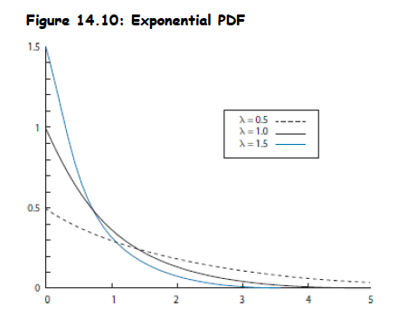
Topic 4. The Exponential distribution
- Definition: Often used to model waiting times. Examples include time taken for an employee to serve a customer or time taken for a company to default.
- PDF:
-
Parameters:
- Scale parameter (β), which is greater than zero.
- Rate parameter (λ), which is the reciprocal of β (λ = 1/β). It measures the rate at which an event will occur (e.g., hazard rate for default).
- Mean of exponential distribution is 1/λ and its variance is .
- The number of defaults up to a certain period ( ) follows a Poisson distribution with a rate parameter equal to t/β
1/\lambda^2
N_t
f(x)=\frac{1}{\beta} x e^{-x / \beta}, x \geq 0
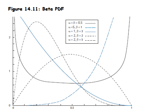
Topic 5. The Beta distribution
- Definition: A distribution whose mass is located between the intervals zero and one.
- Common Occurrences: Can be used for modeling default probabilities and recovery rates. Used in credit risk models like CreditMetrics®.
- Properties: Can be symmetric or skewed depending on the values of its shape parameters (β and α)
Topic 6. Mixture distributions
- Definition: Combine concepts of parametric and nonparametric distributions.
- Characteristics and Creation: Component distributions used as inputs are parametric, while the weights of each distribution within the mixture are based on historical (nonparametric) data. Various distributions can be combined to create unique PDFs.
- Mixing distributions allows modification of skewness by combining distributions with different means and kurtosis by combining distributions with different variances.
- Combining distributions with significantly different means creates mixture distributions with multiple modes, such as bimodal distributions.
QA 3. Common Univariate Random Variables
By Prateek Yadav


