Book 1. Market Risk
FRM Part 2
MR 9. Empirical Properties of Correlation
Presented by: Sudhanshu
Module 1. Empirical Properties of Correlation
Module 1. Empirical Properties of Correlation
Topic 1. Empirical Behaviour of Equity Correlations and Correlation Volatilities
Topic 2. Mean Reversion
Topic 3. Autocorrelation
Topic 4. Best-Fit Distributions for Correlations

Topic 1. Empirical Behaviour of Equity Correlations and Correlation Volatilities
- Study scope: 30 Dow Jones stocks analyzed monthly over 534 months (1972-2017)
- Calculation scale: 30×30 correlation matrix for each stock per month = 900 correlations monthly; 480,600 total correlations computed (900 × 534 = 480,600)
- Economic states defined: Expansion (GDP >3.5%), Normal (GDP 0-3.5%), Recession (2 consecutive quarters of negative growth)
- Period breakdown: 6 recessions, 5 expansionary periods, 5 normal periods identified
- Average correlations by state: Recession (37.0%), Normal (33.0%), Expansion (27.5%)
- Recession behavior: Highest correlations as stocks move down together driven by macroeconomic factors
- Expansion behavior: Lowest correlations; valuations driven more by industry/company-specific factors than macro conditions
- Correlation volatilities: Normal (83.0%), Recession (80.5%), Expansion (71.2%)
- Volatility insight: Highest during normal periods due to directional uncertainty; investors have clearer expectations during recessions (down) and expansions (up)
Practice Questions: Q1
Q1. Suppose a risk manager examines the correlations and correlation volatility of stocks in the Dow Jones Industrial Average (Dow) for the period beginning in 1972 and ending in 2017. Expansionary periods are defined as periods where the U.S. gross domestic product (GDP) growth rate is greater than 3.5%, periods are normal when the GDP growth rates are between 0 and 3.5%, and recessions are periods with two consecutive negative GDP growth rates. Which of the following statements characterizes correlation and correlation volatilities for this sample? The risk manager will most likely find that:
A. correlations and correlation volatility are highest for recessions.
B. correlations and correlation volatility are highest for expansionary periods.
C. correlations are highest for normal periods, and correlation volatility is highest for recessions.
D. correlations are highest for recessions, and correlation volatility is highest for normal periods.
Practice Questions: Q1 Answer
Explanation: D is correct.
Findings of an empirical study of monthly correlations of Dow stocks from 1972 to 2017 revealed the highest correlation levels for recessions and the highest correlation volatilities for normal periods. The correlation volatilities during a recession and normal period were 80.5% and 83.0%, respectively.
Topic 2. Mean Reversion
-
Mean Reversion: Mean reversion implies that, over time, variables or returns regress back to the mean or average return. It is statistically defined as a negative relationship between the change in a variable over time, St−St−1, and the variable in the previous period, St−1.
-
Empirical studies suggests that bond values, interest rates, credit spreads, stock returns, volatility, and other variables are mean reverting.
-
For example, during a recession, demand for capital is low. Therefore, interest rates are lowered to encourage investment in the economy. Then, as the economy picks up, demand for capital increases and, at some point, interest rates will rise. If interest rates are too high, demand for capital decreases and interest rates decrease and approach the long-run average.
-
Mean Reversion Rate (a): The degree of attraction back to the mean, also known as the speed or gravity of mean reversion.
-
The simplified mean reversion rate equation (assuming Δt=1 and ignoring the stochastic term) is:St−St−1=a(μ−St−1)
where St is the value at time t, St−1 is the value in the previous period, and μ is the long-run mean.
-
-
Estimation: The mean reversion rate, a, can be estimated using standard regression analysis. By reformulating the mean reversion equation as:
St−St−1=aμ−aSt−1 , it fits the standard regression form Y=α+βX.
-
A regression is run where Y=St−St−1 is regressed with respect to X=St−1.
-
The β coefficient of the regression is equal to the negative of the mean reversion rate, a.
-
- Example from Dow Stocks: A study using Dow stock data from 1972 to 2017 resulted in the regression equation Y=0.256−0.7903X.
-
The β coefficient of −0.7903 implies a mean reversion rate of 79.03%.
-
Topic 2. Mean Reversion
Practice Questions: Q2
Q2. Suppose mean reversion exists for a variable with a value of 30 at time period t − 1. Assume that the long-run mean value for this variable is 40 and ignore the stochastic term included in most regressions of financial data. What is the expected change in value of the variable for the next period if the mean reversion rate is 0.4?
A. −10.
B. −4.
C. 4.
D. 10.
Practice Questions: Q2 Answer
Explanation: C is correct.
The mean reversion rate, a, indicates the speed of the change or reversion back to the mean. If the mean reversion rate is 0.4 and the difference between the last variable and long-run mean is 10 (= 40 − 30), the expected change for the next period is 4 (i.e., 0.4 × 10 = 4).
Practice Questions: Q3
Q3. A risk manager uses the past 480 months of correlation data from the Dow Jones Industrial Average (Dow) to estimate the long-run mean correlation of common stocks and the mean reversion rate. Based on historical data, the long-run mean correlation of Dow stocks was 32%, and the regression output estimates the following regression relationship: Y = 0.24 − 0.75X. Suppose that in April 2014, the average monthly correlation for all Dow stocks was 36%. What is the expected correlation for May 2014 assuming the mean reversion rate estimated in the regression analysis?
A. 32%.
B. 33%.
C. 35%.
D. 37%.
Practice Questions: Q3 Answer
Explanation: B is correct.
There is a −4% difference from the long-run mean correlation and April 2014 correlation (32% − 36% = −4%). The inverse of the β coefficient in the regression relationship implies a mean reversion rate of 75%. Thus, the expected correlation for May 2014 is 33.0%:
\begin{aligned}
& S_t=a\left(\mu-S_{t-1}\right)+S_{t-1} \\
& S_t=0.75(32 \%-36 \%)+0.36=0.33
\end{aligned}
- Autocorrelation measures the degree that a current variable value is correlated to past values. It measures the persistence to pull toward more recent historical values, having the exact opposite properties of mean reversion.
-
Modeling Autocorelation:
-
Autocorrelation is often calculated using an autoregressive conditional heteroskedasticity (ARCH) model or a generalized autoregressive conditional heteroskedasticity (GARCH) model.
-
The sum of the mean reversion rate and the one-period autocorrelation rate will always equal 1.
-
Example from Dow Stocks: Since the mean reversion rate for Dow stocks in the study was 78%, the autocorrelation for a one-period lag is 22%
-
Autocorrelation for a one-period lag is statistically defined as:
- For Dow stocks example, the autocorrelation calculated using this equation is 20.97%, which is close to 22%. This is the value calculated after subtracting mean-reversion rate (78%) from 1 (=1-78%=22%)
-
Autocorrelations decay with longer time period lags.
-
A C\left(\rho_t, \rho_{t-1}\right)=\frac{\operatorname{Cov}\left(\rho_t, \rho_{t-1}\right)}{\sigma_{\rho_t} \cdot \sigma_{\rho_{t-1}}}
Topic 3. Autocorrelation
Practice Questions: Q4
Q4. A risk manager uses the past 480 months of correlation data from the Dow Jones Industrial Average (Dow) to estimate the long-run mean correlation of common stocks and the mean reversion rate. Based on this historical data, the long-run mean correlation of Dow stocks was 34%, and the regression output estimates the following regression relationship: Y = 0.262 − 0.77X.
Suppose that in April 2014, the average monthly correlation for all Dow stocks was 33%. What is the estimated one-period autocorrelation for this time period based on the mean reversion rate estimated in the regression analysis?
A. 23%.
B. 26%.
C. 30%.
D. 33%.
Practice Questions: Q4 Answer
Explanation: A is correct.
The autocorrelation for a one-period lag is 23% for the same sample. The sum of the mean reversion rate (77% given the beta coefficient of −0.77) and the one period autocorrelation rate will always equal 100%.
Topic 4. Best-Fit Distributions for Correlations
-
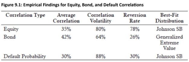
Empirical findings for equity, bond, and default probability correlations:
-
Equity Correlation Distribution Analysis (1972-2017)
-
Positive correlations: 77% of Dow stock pairs showed positive correlation
- Best-fit distribution: Johnson SB distribution (2 shape, 1 location, 1 scale parameter) across all economic states
- Testing methods: Kolmogorov-Smirnov, Anderson-Darling, and chi-squared tests confirmed best fit
- Poor fits: Normal, lognormal, and beta distributions inadequate for equity correlations
- Recession analysis: 3 mild (1980, 1990-91, 2001) and 3 severe recessions (1973-74, 1981-82 oil shocks; 2007-09 financial crisis)
- Pre-recession pattern: correlation volatility decreased before all recessions except 1990-91; consistent with low volatility during expansionary periods
-
Topic 4. Best-Fit Distributions for Correlations
-
Bond and Default Probability Correlations
-
Bond Correlations analyzed: 7,645
- Average correlation: 42% (higher than equities at 37%)
- Correlation volatility: 64%
- Mean reversion rate: 26%
- Best-fit distributions: Generalized extreme value (GEV) primary; normal distribution also fits well
-
Default Probability Correlations analyzed: 4,655
- Average correlation: 30% (lowest of three asset classes)
- Correlation volatility: 88% (highest volatility)
- Mean reversion rate: 30% (similar to bonds at 26%)
- Best-fit distribution: Johnson SB (same as equities, different from bonds)
-
Practice Questions: Q5
Q5. In estimating correlation matrices, risk managers often assume an underlying distribution for the correlations. Which of the following statements most accurately describes the best-fit distributions for equity correlation distributions, bond correlation distributions, and default probability correlation distributions? The best-fit distribution for the equity, bond, and default probability
correlation distributions, respectively, are:
A. lognormal, generalized extreme value, and normal.
B. Johnson SB, generalized extreme value, and Johnson SB.
C. beta, normal, and beta.
D. Johnson SB, normal, and beta.
Practice Questions: Q5 Answer
Explanation: B is correct.
Equity correlation distributions and default probability correlation distributions are best fit with the Johnson SB distribution. Bond correlation distributions are best fit with the generalized extreme value distribution.
MR 9. Empirical Properties of Correlation
By Prateek Yadav


