Book 2. Credit Risk

FRM Part 2

CR 19. Future Value and Exposure

Presented by: Sudhanshu

Module 1. Credit Exposure

Module 2. Security Exposure Profiles

Module 3. Collateral and Credit Exposure

Module 1. Credit Exposure

Topic 1. Credit Exposure Metrics

Topic 2. Credit Exposure Vs. VaR Methods

Topic 3. Credit Exposure Factors

Topic 1. Credit Exposure Metrics

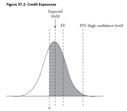
• Expected Mark-to-Market (MtM): Expected value of a transaction at a future point in time; long measurement periods and specific cash flow characteristics can create large differences between current and expected MtM
• Expected Exposure (EE): Amount expected to be lost if there is positive MtM and the counterparty defaults; larger than expected MtM because it considers only positive MtM scenarios (not negative values)
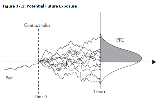
• Potential Future Exposure (PFE): Worst-case MtM estimate at a specific future point based on a high confidence level
  • Derived from a probability distribution of possible future MtM paths
  • Represents positive MtM exposure at risk if counterparty defaults
  • Maximum PFE is the highest PFE value over a stated time frame

Topic 1. Credit Exposure Metrics

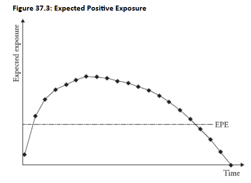
• Expected Positive Exposure (EPE): Average of expected exposure through time; provides a useful single measure to quantify exposure over the life of transactions
• Expected Negative Exposure (ENE): Opposite of EPE; represents exposure from the counterparty's perspective based on negative future values
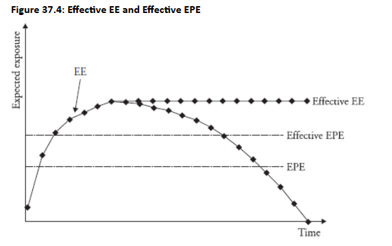
• Effective EE and Effective EPE: Designed to capture rollover risk for short-term transactions (under one year)
  • Effective EE equals non-decreasing EE (prevents exposure from declining)
  • Effective EPE is the average of effective EE

Practice Questions: Q1

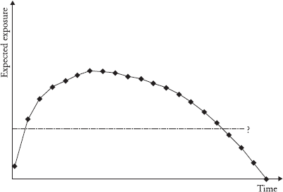
Q1. Which metric for credit exposure is represented by the “?” in the following graph?

A. Expected positive exposure (EPE).
B. Potential future exposure (PFE).
C. Effective expected exposure (EE).
D. Effective expected positive exposure (EPE).

Practice Questions: Q1 Answer

Explanation: A is correct.

EPE is equal to average EE over time. It is a useful single amount to quantify exposure.

Topic 2. Credit Exposure Vs. VaR Methods

• Value at Risk (VaR) Definition: Measures the estimated risk of loss on a financial/investment portfolio; example: one-day 10% VaR of $100,000 means a 10% probability the portfolio will fall by more than $100,000 in one day
• Application Differences:
  • Credit exposure is defined for both pricing and risk management, making quantification more difficult with potentially different calculations for each purpose
  • VaR is used only for risk management
• Time Horizon Considerations:
  • VaR uses relatively short time horizons where drift, volatility trends, and co-dependence of market variables are largely irrelevant
  • Credit exposure must be defined over many time horizons, making drift, volatility, and co-dependence critical factors
  • Credit exposure must account for future contractual payments, exercise decisions, cash flows, and cancellations that create path dependency, whereas VaR typically ignores these elements
• Risk Mitigants: Credit exposure estimation must incorporate netting and collateral as risk reduction mechanisms; netting requires complex rule applications, while future collateral introduces subjectivity in modeling type and timing despite uncertain variables

Topic 3. Credit Exposure Factors

• Future Uncertainty: In contracts with single payouts at maturity (e.g., FX forwards, FRAs), uncertainty regarding the final exchange value increases over time, elevating credit exposure
• Periodic Cash Flows: Regular cash flows reduce the negative impact of future uncertainty, though additional risk exists when periodic payments are unequal and based on variable factors (e.g., floating-rate interest rate swaps)
• Combination of Profiles: Credit exposure results from multiple underlying risk factors combined in a single product (e.g., cross-currency swaps combining FX forward and interest rate swap components)
• Optionality: Exercise decisions embedded in derivative contracts (e.g., swaptions) significantly impact credit exposure levels
• Collateral Impact: While collateral typically reduces credit exposure, true risk reduction depends on:
  • Key parameters (minimum transfer amounts, thresholds)
  • Margin period of risk
  • Associated risks (liquidity, operational, legal)
• Collateral Limitations: Risk is not entirely eliminated even with collateral due to:
  • Delays in receiving collateral
  • Variations in collateral value (non-cash collateral)
  • Granularity effect (parameters prevent requesting full required collateral)
  • Path dependency (amount called depends on past collection history)

Module 2. Security Exposure Profiles

Topic 1. Typical Credit Exposure Profiles

Topic 2. Impact of Payment Frequencies & Exercise Dates

Topic 3. Modeling Netting & Collateral

Topic 1. Typical Credit Exposure Profiles

• PFE Definition: Maximum expected credit risk exposure for a specified period at a prespecified confidence level (typically 99%); represents the upper bound on a confidence interval for future counterparty credit risk exposure
• Time Impact: Ability to quantify counterparty credit exposure is affected by time to maturity, with greater uncertainty for market variables further into the future
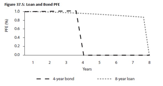
• Bonds and Loans (Fig 37.5):
  • PFE approximately equals notional value for bonds, loans, and repos
  • Four-year bond shows additional exposure from interest rate risk (fixed-rate bonds increase exposure when rates decline)
  • Eight-year loan exposure may decrease over time due to variable rates and prepayments

Topic 1. Typical Credit Exposure Profiles

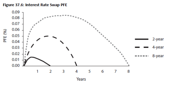
• Swaps (Fig 37.6): Exposure profiles exhibit a characteristic peak shape, resulting from the balance between future payment uncertainties and roll-off risk of swap payments over time
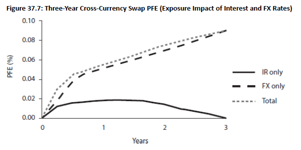
• Foreign Exchange Products (Fig 37.7): High FX volatility, long maturities, and large final notional payments create monotonically increasing exposures; majority of exposure comes from FX rate uncertainty rather than interest rate risk

Topic 1. Typical Credit Exposure Profiles

• Long Option Positions (Fig 37.8): Exposure increases over time until exercise (with up-front premium paid); shape varies based on whether option is in, at, or out of the money, but time increase is similar as options can move deep in the money
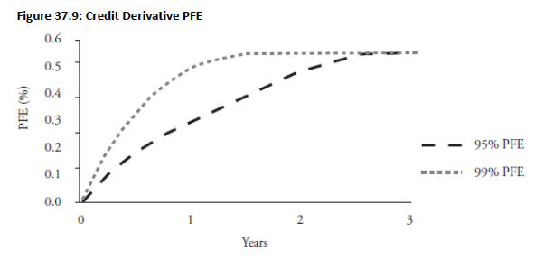
• Credit Default Swaps (Long Protection) (Fig 37.9):
  • Wrong-way risk creates considerable counterparty risk
  • Early-year exposure increase results from CDS premium/credit spread widening
  • Maximum exposure occurs at credit event (notional value minus recovery value)
  • Example shows 55% final exposure based on 45% recovery rate assumption

Topic 2. Impact of Payment Frequencies & Exercise Dates

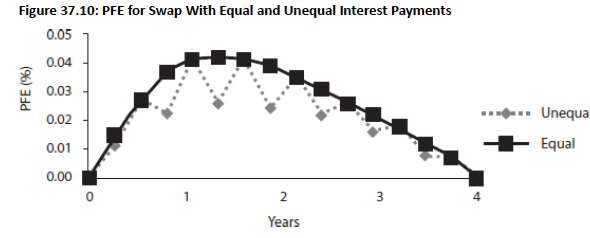
• Impact of Payment Frequencies (Fig 37.10):

  • In an interest rate swap with semiannual fixed payments made and quarterly floating payments received, exposure is reduced when payments are received more frequently than payments are made

  • Reverse effect occurs when payments made are more frequent than payments received (unequal payment PFE shows greater exposure than equal payment PFE)

Topic 2. Impact of Payment Frequencies & Exercise Dates

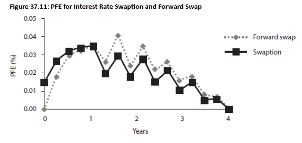
• Impact of Exercise Date (Fig 37.11): Exposure profile for a swap-settled interest rate swaption versus forward swap with one-year exercise date shows distinct patterns:

  • Pre-Exercise Period: Swaption exposure is greater than forward swap exposure before the one-year exercise date
  • Post-Exercise Period: Relationship reverses; forward swap exposure exceeds swaption exposure because in some scenarios the forward swap has positive value while the swaption is not exercised
  • Payment frequencies also differ between the swaps in this comparison

Practice Questions: Q2

Q2. Which of the following security types will most likely result in a peaked shape for the exposure profile represented by potential future exposure (PFE)?
A. Long option position.
B. Foreign exchange product.
C. 10-year loan with a floating rate payment.
D. Swap.

Practice Questions: Q2 Answer

Explanation: D is correct.

Exposure profiles of swaps are typically characterized by the peaked shape that results from balancing future uncertainties over payments and roll-off risk of swap payments over time.

Topic 3. Modeling Netting & Collateral

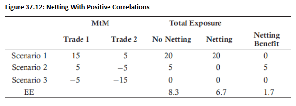
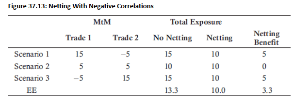
• Netting Mechanism: Netting agreements allow two parties to offset positions upon default; benefits realized when mark-to-market (MtM) values have opposite signs, calculated at individual level before computing total expected exposure (EE)
• Exposure Metrics: Single time horizon netting factor defined by EE; weighted average EE over time defines expected positive exposure (EPE)
• Netting Factor Formula:
  •  
  •  
    • where n = number of exposures and      = average correlation
    • 100% netting factor = no netting benefit (correlation = 1)
    • 0% netting factor = maximum netting benefit
• Netting Factor Behavior: Netting benefit improves (i.e., netting factordeclines) with larger number of exposures and lower correlation. 
  • ​If correlation = 0 =>
    • ​=> For 2 independent exposures, netting factor =71%
• Initial MtM Dependency:
  • Trades with strong negative MtM under all scenarios enhance netting benefit by offsetting positive MtM of other trades
  • Trades with strong positive exposure under all scenarios reduce netting benefit by offsetting negative MtM of other trades

Topic 3. Modeling Netting & Collateral

• Correlation Impact on Netting:
  • Positive correlations provide lower netting benefits (trades likely same sign, minimal offsetting)
  • Perfect positive correlation provides least netting benefit
  • Negative correlations provide stronger netting benefits (trades offset each other)
  • Perfect negative correlation yields maximum 100% netting benefit with zero overall risk

Practice Questions: Q1

Q1. Miven Corp. has two trades outstanding with one of its counterparties. Which of the following scenarios would result in the greatest netting advantage for Miven?
A. The two trades have strong positive correlation.
B. The two trades have weak positive correlation.
C. The two trades are uncorrelated with each other.

D. The two trades have strong negative correlation.

Practice Questions: Q1 Answer

Explanation: D is correct.

The greatest netting benefit among the scenarios presented occurs when the two trades have a strong negative correlation. In this case, a large portion of the negative exposures will offset positive exposures.

Practice Questions: Q3

Q3. Which of the following statements best describes the benefit of netting risk exposures? The benefits of netting are realized when:
A. marked-to-market (MtM) values have high structural correlations for two trades.
B. marked-to-market (MtM) values have opposite signs for two trades.
C. expected exposure (EE) values are minimal.
D. expected future exposure (EFE) values have zero correlation.

Practice Questions: Q3 Answer

Explanation: B is correct.

The benefits of netting are realized when MtM values have opposite signs for two trades.

Module 3. Collateral and Credit Exposure

Topic 1. Margin Period of Risk (MPOR)

Topic 2. Modeling Collateral

Topic 3. Funding Exposure Vs. Credit Exposure

Topic 4. Impact of Collateral on Counterparty Risk and Funding

Topic 1. Margin Period of Risk (MPOR)

• Credit Exposure Direction: When Party A has positive exposure (receives cash flows from Party B), Party A faces credit risk if Party B defaults; when exposure is negative, Party A must post collateral to Party B to minimize credit risk
• Collateral Risk Reduction Factors: Risk managers must understand factors affecting collateral's ability to reduce risk, including thresholds, minimum transfer amounts, rounding, initial margin, and margin period of risk
• MPoR Definition: The period from when a collateral call occurs to when collateral is actually delivered; represents extreme exposure to the counterparty, with prudent analysts assuming counterparty default during this period
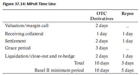
• MPoR Calculation Steps:
  • Step 1 - Valuation/Margin Call: Time to calculate current exposure and collateral market value to determine validity of call
  • Step 2 - Receiving Collateral: Period between counterparty receiving request and releasing collateral
  • Step 3 - Settlement: Time to sell collateral for cash (varies by security type: cash intraday, government bonds 1 day, corporate bonds 3 days)
  • Step 4 - Grace Period: Time allowed before counterparty is considered in default for failure-to-pay
  • Step 5 - Liquidation/Close-out and Re-hedge: Time needed to liquidate collateral, close out positions, and re-hedge

Topic 1. Margin Period of Risk (MPOR)

• MPoR Determinants (Fig 37.14): An example of a MPoR time line is found in Fig 37.14, along with the minimum period lengths that must be assumed according to Basel II.
  • Length depends on collateral agreement terms, counterparty characteristics, legal considerations, and institutional management structure
  • Basel II establishes minimum period lengths separately for OTC derivatives and repos due to different documentation requirements
  • Requesting party may show leniency to maintain business relationships

Practice Questions: Q1

Q1. Time steps that enter into the calculation of the number of days in the margin period of risk include all of the following except:
A. valuation/margin call.
B. posting collateral.
C. settlement.
D. close-out and re-hedge.

Practice Questions: Q1 Answer

Explanation: B is correct.

The time period from which the request for collateral is received to which it is released refers to the receipt of collateral, but it does not involve its actual posting. All of the remaining items are part of the MPoR.

Topic 2. Modeling Collateral

• Imperfect Collateralization: Collateral agreement terms (threshold, minimum transfer amount, rounding) may result in less than full collateralization. The following expression represents imperfect collateralization:

  •  

  • where

    • ​t = time

    •  

• Exposure Increases Between Margin Calls: Exposure can grow between collateral calls, creating uncollateralized portions where current exposure exceeds previous exposure levels

  • ​

• Path Dependency: Amount of collateral requested depends on historical collateral collection amounts, creating dependency on past margin calls

Topic 2. Modeling Collateral

• Key Parameters Affecting Collateral Effectiveness:

  • Margin Period of Risk (MPoR): Time lag between calling for collateral and actually receiving it
  • Threshold: Exposure level below which no collateral is called, representing permanent uncollateralized exposure
  • Minimum Transfer Amount: Smallest block size for collateral transfers; amounts below this remain uncollateralized
  • Initial Margin (Independent Amount): Amount posted upfront, independent of subsequent collateral calls
  • Rounding: Adjustment of collateral call amounts to specific increments, potentially leaving gaps in coverage

Topic 3. Funding Exposure Vs. Credit Exposure

• Funding Costs and Benefits:

  • Counterparty default creates potential positive credit exposure, resulting in funding cost to the firm
  • Firm's own default creates potential negative credit exposure, resulting in funding benefit
  • Posting margin against positive exposure decreases both funding costs and counterparty risk
  • Posting margin against negative exposure decreases both funding benefits and counterparty's exposure
• Key Differences between Credit Exposure and Funding Exposure:
  • Defining Value: Credit exposure value is subjective and depends on close-out procedure assumptions; funding exposure value is objective as it exists in non-defaulting situations
  • Margin Period of Risk: Credit exposure assumes counterparty default in calculations; funding exposure considers funding delay without necessarily assuming default, so funding value adjustment (FVA) can be zero even when credit value adjustment (CVA) is non-zero
  • Aggregation: Credit exposure focuses on netting values at default; funding exposure considers the entire portfolio as margin from different counterparties can be reused
  • Wrong-Way Risk: Relevant concept for measuring credit exposure but not a key consideration for funding exposure
  • Segregation: Restricts margin usage, impacting credit and funding exposure differently

Topic 4. Impact of Collateral on Counterparty Risk and Funding

• Cash (Not Segregated): Mitigates both counterparty risk and funding costs; optimal collateral type for dual benefit
• Securities (Rehypothecatable): Mitigates both counterparty risk and funding costs, provided haircuts are sufficient to cover potential value fluctuations
• Cash and Securities (Segregated, Non-Rehypothecatable): Mitigates counterparty risk but provides no funding benefits since collateral cannot be reused in non-default scenarios
• Counterparty Bonds (Rehypothecatable): Mitigates funding costs but problematic for counterparty risk mitigation due to wrong-way risk (bonds will be in default precisely when needed)
• Optimal Collateral Characteristics: To maximize both counterparty risk mitigation and funding benefits, collateral must:
  • Not exhibit wrong-way risk
  • Be reusable (not segregated)

• Collateral Benefits: Counterparty risk is reduced by taking ownership of collateral upon default and funding costs are mitigated by posting collateral against other transactions
• Optimal Collateral Characteristics: To maximize both counterparty risk mitigation and funding benefits, collateral must:
  • Not exhibit wrong-way risk
  • Be reusable (i.e., not segregated)
• Impact of Collateral Types: The impact of different types of collateral on counterparty risk and funding costs can be examined under the following scenarios:
  • Cash (Not Segregated): Mitigates both counterparty risk and funding costs; optimal collateral type for dual benefit
  • Securities (Rehypothecatable): Mitigates both counterparty risk and funding costs, provided haircuts are sufficient to cover potential value fluctuations
  • Cash and Securities (Segregated, Non-Rehypothecatable): Mitigates counterparty risk but provides no funding benefits since collateral cannot be reused in non-default scenarios
  • Counterparty Bonds (Rehypothecatable): Mitigates funding costs but problematic for counterparty risk mitigation due to wrong-way risk (bonds will be in default precisely when needed)

Topic 4. Impact of Collateral on Counterparty Risk and Funding