Book 2. Credit Risk
FRM Part 2
CR 12. Credit Risk
Presented by: Sudhanshu
Module 1. Default Probabilities
Module 2. Credit Risk in Derivatives
Module 3. Default Correlation and Credit VaR
Module 1. Default Probabilities

Topic 1. Credit Risk and Default Probability
Topic 2. Default Probabilities Using Credit Spreads
Topic 3. Default Probability Estimate Comparisons
Topic 4. Equity Prices for Default Probability Estimates
Topic 1. Credit Risk and Default Probability
-
Credit Risk: Credit risk is the exposure an entity faces from the potential default of a counterparty in a derivatives contract or a borrower.
-
Key Factors: Credit ratings, default probabilities, and recovery rates.
-
-
Credit Rating Agencies: Moody's, S&P, and Fitch provide corporate bond ratings.
-
Investment Grade vs. Lower Rated Bonds: Bonds rated Baa and above (by Moody's) are considered investment grade and have significantly lower default probabilities than lower-rated bonds.
- Investment-grade bonds may experience deteriorating financial health over time, while non-investment-grade bonds may improve in credit quality after surviving the critical early years.
- Unconditional Default Probability: Probability of default in a given year, seen today.
-
Hazard Rate (Default Intensity): A measure of conditional probability of default, Q(t).
-
-
Recovery Rate: For a bond, it is market value post-default divided by its face value.
-
Higher for first and second lien bonds versus those for subordinated bonds
- Corporate bond recovery rates show negative dependence on default rates: strong economic conditions lead to fewer defaults and higher recoveries, while weak conditions result in more defaults and lower recoveries.
-
\mathrm{Q}(\mathrm{t})=1-\mathrm{e}^{-\bar{\lambda}(\mathrm{t}) \times \mathrm{t}}; \text{ where }
\bar{\lambda}(\mathrm{t})= \text{average hazard rate between time 0 and time }t
-
Relationship over time:
-
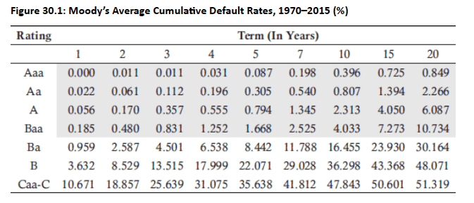
For a bond rated Baa, the probability of default in Year 3 is 0.831% − 0.480% = 0.351%. In Year 4, it is 1.252% − 0.831% = 0.421% (which is higher than in Year 3).
-
For a bond rated B, the probability of a Year 3 default is: 13.515% − 8.529% = 4.986%. For Year 4, it is 17.999% − 13.515% = 4.484% (which is lower than in Year 3).
-
Conclusion: Investment-grade bonds may experience deteriorating financial health over time, while non-investment-grade bonds may improve in credit quality after surviving the critical early years (as stated earlier).
-
Topic 1. Credit Risk and Default Probability
-
For a B-rated bond,
-
The unconditional default probability during Year 4: is calculated as the difference between the 4-year and 3-year cumulative default rates: 17.999%−13.515%=4.484%.
-
Probability of survival through Year 3: 100% − 13.515% = 86.485%
-
Conditional probability of a default during Year 4, (conditional on no earlier default): 0.04484/0.86485 = 5.185%
-
Topic 1. Credit Risk and Default Probability
Practice Questions: Q1
Q1.If the unconditional default probability of a Ba-rated bond during Year 3 is 1.914% and the probability of survival through Year 2 is 97.413%, the probability of a default during Year 3, conditional on no earlier default, is closest to:
A. 0.673%.
B. 1.914%.
C. 1.965%.
D. 2.587%.
Practice Questions: Q1 Answer
Explanation: C is correct.
The probability of a default during Year 3, conditional on no earlier default, is
equal to: 0.01914/0.97413 = 1.965%.
Topic 2. Default Probabilities Using Credit Spreads
- Yield Spread: The yield spread of a bond is the difference between its promised yield and the risk-free rate.
-
Hazard Rate Approximation: The average hazard rate, , can be approximated using the bond yield spread, s(T), and the recovery rate, RR.
-
-
-
-
Example: A one-year bond with a 125 basis point spread over the risk-free rate and a 55% recovery rate has an average hazard rate of: 0.0125/(1−0.55)=0.0278, or 2.78% per year.
-
Increasing precision: Greater precision is achieved by aligning hazard rates with bond prices, where the first period hazard rate uses the shortest maturity bond, the next period uses the next shortest maturity, and so on.
-
Risk-Free Rate: It is often proxied by a Treasury rate. However, there is concern that these rates are too low to truly proxy risk-free rates. Below alternatives can be used:
-
CDS spreads can be used as they do not depend on the risk-free rate.
-
An asset swap spread can also be used, as the PV of the spread is the difference between the price of the risk-free bond and the price of the corporate bond.
-
\bar{\lambda}(T)
\bar{\lambda}(T)=\frac{s(T)}{1-RR}
Practice Questions: Q2
Q2. A 2-year corporate bond yields 190 basis points above the risk-free rate. With a recovery rate of 35%, the average hazard rate for Years 1 and 2 is closest to:
A. 0.67%.
B. 1.55%.
C. 2.92%.
D. 5.43%.
Practice Questions: Q2 Answer
Explanation: C is correct.
A 2-year bond yielding 190 basis points above the risk-free rate with a recovery rate of 35% would yield an average hazard rate of: 0.0190/(1 − 0.35) = 0.0292, or 2.92% per year.
Topic 3. Default Probability Estimate Comparisons
-
Bond Yield Spreads vs. Historical Data Estimates:
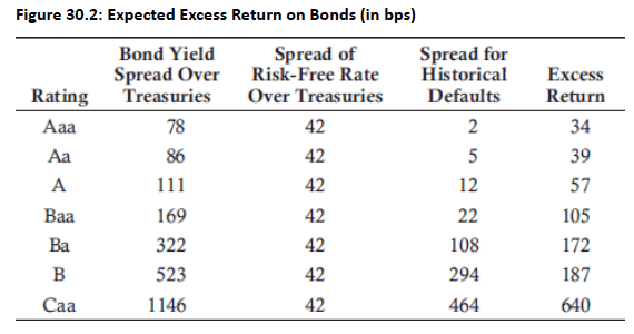
- Higher Estimates: Bond yield spreads generally produce higher estimated default probabilities than historical data. This difference becomes even more significant during economic crises.
- Expected Excess Return: The table below shows the expected excess return on bonds (in basis points) for spreads over Treasuries at various rating categories.
- Rating and Hazard Rates: For investment-grade companies, the ratio of the hazard rate from bond prices to the hazard rate from historical data is very high, but this ratio decreases as credit ratings decline. This leads to to an increase in the spread between the hazard rates.
Topic 3. Default Probability Estimate Comparisons
-
Real-World vs. Risk-Neutral Probabilities:
- Risk-Neutral Probabilities: These are implied from credit spreads and are used for pricing instruments and valuing credit derivatives.
- Real-World Probabilities: These are based on real-world (physical) historical data and are used for scenario analysis to calculate potential future losses.
-
Difference: Risk-neutral probabilities are typically higher than real-world probabilities due to below reasons.
- This difference is mainly due to the systematic risk of bond defaults, which cannot be diversified away.
- Other factors include the relative illiquidity of corporate bonds and the subjective probabilities of bond traders.
Topic 4. Equity Prices for Default Probability Estimates
-
The Merton Model
-
Equity as an Option: The Merton model views a company's equity as a call option on the company's asset value, with the strike price being the required debt repayment (D).
-
-
Value of Equity: The value of equity today (E0) can be calculated using the Black-Scholes-Merton formula.
-
-
Value of Debt: The value of debt today (D0) is the difference between the company's asset value and its equity value (D0=V0−E0).
-
Example: Suppose the market value of debt, calculated as V0−E0V_0 - E_0V0−E0, is 8.25, while the present value of the promised debt payment equals 8.41.
-
Model Accuracy: Historical data suggests that the Merton model produces solid rankings of default probabilities in both risk-neutral and real-world scenarios
-
E_T=max(V_T-D,0)
\begin{aligned}
&\mathrm{E}_0=\mathrm{V}_0 \mathrm{~N}\left(\mathrm{~d}_1\right)-\mathrm{D} \mathrm{e}^{-\mathrm{rT}} \mathrm{~N}\left(\mathrm{~d}_2\right); \text { where, }\\
&\begin{aligned}
& \mathrm{d}_1=\frac{\ln \left(\mathrm{V}_0 / \mathrm{D}\right)+\left(\mathrm{r}+\sigma_{\mathrm{v}}^2 / 2\right) \mathrm{T}}{\sigma_{\mathrm{v}} \sqrt{\mathrm{~T}}}; \mathrm{~d}_2=\mathrm{d}_1-\sigma_{\mathrm{v}} \sqrt{\mathrm{~T}}
\end{aligned}
\end{aligned}
Module 2. Credit Risk in Derivatives
Topic 1. Credit Risks of Derivatives
Topic 2. CVA and DVA
Topic 3. Credit Risk Mitigation
Topic 1. Credit Risks of Derivatives
-
ISDA Master Agreement: The International Swaps and Derivatives Association (ISDA) Master Agreement is typically used to govern bilaterally cleared derivatives transactions between two companies.
-
ISDA agreement outlines initial and variation margin requirements for financial institutions and defines what constitutes an "event of default".
-
Transactions are netted for only variation margin calculations.
-
-
Risk for Non-Defaulting Party: A non-defaulting party in a derivatives transaction will likely incur a loss in two primary situations.
-
The total value of the transactions for the non-defaulting party is positive and exceeds the collateral posted by the defaulting party. In this case, the non-defaulting party becomes an unsecured creditor for the amount of the transactions minus the collateral.
-
The total value of the transactions for the defaulting party is positive and is less than the collateral posted by the non-defaulting party. Here, the non-defaulting party becomes an unsecured creditor for the return of the excess collateral they posted.
-
Practice Questions: Q1
Q1. In a bilaterally cleared derivatives transaction between two companies (Company A and Company B), Company B defaults. The value for Company A is a positive $50,000 and the collateral posted by Company B is $30,000. In this situation, Company A is a(n):
A. secured creditor in the amount of $20,000.
B. secured creditor in the amount of $80,000.
C. unsecured creditor in the amount of $20,000.
D. unsecured creditor in the amount of $80,000.
Practice Questions: Q1 Answer
Explanation: C is correct.
The total value for Company A (as the nondefault party) is positive, and at $50,000, it exceeds the $30,000 collateral posted by Company B (as the default party). Company A will be an unsecured creditor for an amount equal to $50,000 −$30,000 = $20,000.
Topic 2. CVA and DVA
- CVA (Credit Valuation Adjustment): From a bank's perspective, CVA is the present value of the expected cost to the bank if its counterparty defaults.
-
DVA (Debt Valuation Adjustment): DVA is the present value of the expected cost to the counterparty if the bank itself defaults.
-
CVA and DVA as derivatives: CVA and DVA can be considered derivatives, which change in value due to market variables, counterparty credit spreads, and bank credit spreads.
-
DVA as a Benefit: A bank's default means it won't have to make payments on its derivatives positions, so DVA is considered a benefit to the bank, increasing the value of its portfolio.
-
Valuing the Portfolio: The total value of a bank's derivatives transactions, accounting for the possibility of default, is calculated as the no-default value minus CVA plus DVA:
-
-
Wrong-Way & Right-Way Risk:
-
Wrong-way risk occurs when the probability of default is positively correlated with exposure.
-
Right-way risk occurs when the probability of default is negatively correlated with exposure.
-
V_{Portfolio}=f_{nd}-CVA+DVA
-
CVA and DVA Calculations
-
-
- : PV of the expected loss to the counterparty (which is a gain to the bank) if the bank defaults at the midpoint of the ith interval.
-
: The risk-neutral probability of the bank defaulting during the ith interval, calculated from the bank's credit spreads.
-
: PV of the expected loss to the bank if the counterparty defaults at the midpoint of the ith interval.
-
: The risk-neutral probability of the counterparty defaulting during the ith interval.
- Also,
-
-
v_i^{*}
q_i^{*}
v_i
q_i
Topic 2. CVA and DVA
\begin{aligned}
\mathrm{q}_{\mathrm{i}}&=\exp \left(-\frac{\mathrm{s}\left(\mathrm{t}_{\mathrm{i}-1}\right) \mathrm{t}_{\mathrm{i}-1}}{1-\mathrm{RR}}\right)-\exp \left(-\frac{\mathrm{s}\left(\mathrm{t}_{\mathrm{i}}\right) \mathrm{t}_{\mathrm{i}}}{1-\mathrm{RR}}\right) \text{ ; where, }\\
s(t_i)&= \text{counterparty credit spread}
\end{aligned}
CVA=\sum_{i=1}^N q_i \times v_i \text{ ; }DVA=\sum_{i=1}^N q_i^{*} \times v_i^{*} \text{ ; where,}
Topic 2. CVA and DVA
-
Multiple Derivative Positions: Extensive Monte Carlo simulations are often needed to perform CVA and DVA calculations.
-
Peak exposure at the midpoint of each interval in the event of default is an additional calculation banks perform.
-
The impacts of new transactions on CVA and DVA can be calculated quickly as banks often store all sampled paths from their simulations for all market variables.
-
A new transaction, which is positively (negatively) correlated to existing transactions, will likely increase (decrease) CVA and DVA.
-
-
Single (uncollateralized) derivative: Extensive Monte Carlo simulations are not needed.
-
The bank exposure in the future is the no-default derivative value at that time, where the present value is the no-default value today.
-
If DVA=0, the value of the derivative today (accounting for credit risk) is equal to:
-
-
For the value of a T-year zero-coupon bond issued by the counterparty with nd again representing a no-default situation, the value of the bond is equal to:
-
f=f_{\mathrm{nd}}-(1-\mathrm{RR}) f_{\mathrm{nd}} \sum_{\mathrm{i}=1}^{\mathrm{N}} \mathrm{q}_{\mathrm{i}}
\mathrm{B}=\mathrm{B}_{\mathrm{nd}}-(1-\mathrm{RR}) \mathrm{B}_{\mathrm{nd}} \sum_{\mathrm{i}=1}^{\mathrm{N}} \mathrm{q}_{\mathrm{i}}
\implies \frac{f}{f_{\mathrm{nd}}}=\frac{\mathrm{B}}{\mathrm{~B}_{\mathrm{nd}}}
Practice Questions: Q2
Q2. A bank is assessing the impact of a new transaction on CVA and DVA. If the new transaction is negatively correlated to existing transactions, the impact will likely be a(n):
A. increase to both CVA and DVA.
B. decrease to both CVA and DVA.
C. increase to CVA and decrease to DVA.
D. decrease to CVA and increase to DVA.
Practice Questions: Q2 Answer
Explanation: B is correct.
If a new transaction is negatively correlated to existing transactions for the bank and the counterparty, the new transaction will likely decrease both the CVA and the DVA.
Topic 3. Credit Risk Mitigation
-
Key Mitigation Techniques
-
Netting: This reduces exposure by offsetting positive and negative transaction values with a counterparty. For example, if a bank has four uncollateralized transactions with a counterparty with values of +$5M, -$7M, +$10M, and -$2M, the total exposure is not the sum of positive values ($15M) but the net value, which is +$6M.
-
Collateral Agreements: In the event of a default, the non-defaulting party can keep the cash or marketable securities posted as collateral by the defaulting party.
-
Downgrade Triggers: These are clauses in agreements that allow the non-defaulting party (e.g., a bank) to either close out outstanding transactions at market value or demand collateral if the counterparty's credit rating falls below a specified level.
-
The value of these triggers can be reduced by significant rating downgrades or if the counterparty has similar triggers with multiple dealers
-
-
Practice Questions: Q3
Q3. Bank TGF has three uncollateralized transactions with JL Co. The transactions have values to the bank of: +$12 million, −$4 million, and −$3 million. If the bank mitigates its credit risk through netting, the impact of this technique will result in an exposure reduction of:
A. $5 million.
B. $7 million.
C. $8 million.
D. $12 million.
Practice Questions: Q3 Answer
Explanation: B is correct.
If the bank treats all three transactions as individual transactions, the exposure is $12 million. If the transactions are netted, the exposure is $5 million. This equates to an exposure reduction of $7 million.
Module 3. Default Correlation and Credit VaR
Topic 1. Default Correlation for Credit Portfolios
Topic 2. Gaussian Copula Model
Topic 3. Credit VaR
Topic 1. Default Correlation for Credit Portfolios
- Definition: Default correlation is the likelihood that two companies will default around the same time.
-
Causes: Default correlation can be caused by:
-
External events impacting companies in the same region or industry,
-
Overall economic conditions leading to higher average default rates in some years relative to other years.
-
Contagion where one company's default causes another's. Credit risk cannot be fully diversified away due to default correlation.
-
-
Diversification Limits: Because of default correlation, credit risk cannot be fully diversified away.
-
Modeling Approaches: Two main methods are used to model default correlation:
-
Reduced-form models: Assume hazard rates are correlated with macroeconomic variables and follow random processes.
-
Mathematically straightforward and reflect economic cycles,
-
Range of achievable default correlations are low as it is unlikely any two companies will default over the same short period of time.
-
-
Structural models: Based on models like the Merton model.
-
Default correlations are introduced by assuming correlated stochastic processes for the companies' assets.
-
Can be set to have a high correlation but computationally intensive.
-
-
Practice Questions: Q1
Q1. Which of the following statements is most accurate regarding reduced-form versus structural models used to estimate default correlation?
A. Structural models tend to take a long time to process.
B. Reduced-form models are more computationally intensive.
C. Reduced-form models allow for very high default correlations.
D. Economic cycle impacts on default correlation trends are best reflected in structural models.
Practice Questions: Q1 Answer
Explanation: A is correct.
Structural models are computationally intensive (relative to reduced-form models), and, therefore, take a long time to process. However, an advantage to structural models is that they allow for higher default correlations. Economic cycle impacts on default correlation trends are best reflected in reduced-form models.
Topic 2. Gaussian Copula Model
- Modeling Time to Default: The Gaussian copula model is used to quantify the correlation between the probability distributions of times to default for multiple companies. It assumes that all companies will eventually default.
-
Probability Types: Both real-world and risk-neutral default probabilities can be used.
-
Real-world probabilities: The left tail is estimated from rating agency data.
-
Risk-neutral probabilities: The left tail is estimated from bond prices.
-
- Transformation: The model transforms the non-normal times to default into normal variables with zero mean and unit standard deviation.
-
The Copula: The assumption that the joint distribution of these variables is bivariate normal is called the Gaussian copula.
-
It allows the correlation structure to be estimated independently of the unconditional distributions.
-
This default correlation is also known as the copula correlation.
-
- One-Factor Gaussian Copula Model: A one-factor model can be used to avoid needing different correlations for each company pair.
-
Formula: The model assumes that a company's default is impacted by a common factor (F) and a company-specific factor .
-
-
Conditional Default Probability: The default probability for company i by time T, conditioned on the common factor F, is given by:
-
-
When the probability distributions of default are the same for all companies, and the correlations are the same for all companies (i.e., common correlation ρ), the default probability equation can be restated as:
-
-
-
(Z_i)
\begin{aligned}
\mathrm{a}_{\mathrm{i}} &= \text{correlation of company } i \text{ equity returns with a market index}\\
\mathrm{F}&= \text{common factor, which impacts defaults for all companies}\\
\mathrm{Z}&= \text{factor impacting only one company } i \\
\end{aligned}
x_i=a_iF+\sqrt{1-a_i^2}Z_i \text{ ; where }
Q_i(T|F)=N\left(\frac{N^{-1}[Q_i(T)]=a_iF}{\sqrt{1-a_i^2}}\right)
Topic 2. Gaussian Copula Model
Q(T \mid F)=N\left(\frac{N^{-1}[Q(T)]-\sqrt{\rho} F}{\sqrt{1-\rho}}\right)
Practice Questions: Q2
Q2. The Gaussian copula model transforms which of the following factors into normal variables?
A. Recovery rates.
B. Times to default.
C. Credit spread risk.
D. Default probabilities.
Practice Questions: Q2 Answer
Explanation: B is correct.
The Gaussian copula model transforms the times to default into normal variables with means of zero and unit standard deviations. The other choices are all relevant in the credit risk world, but they are not transformed into normal variables via this model.
Topic 3. Credit VaR
- Definition: Credit value at risk (VaR) is the credit risk loss that will not be exceeded over a given period of time, at a specific confidence level.
- Interpretation: A credit VaR with a one-year time horizon and a 98.5% confidence level is the credit loss we are 98.5% confident will not be exceeded over that one-year period of time.
-
Calculation using Gaussian Copula: The percentage of losses on a large portfolio that will be less than V(T,X) is given by the formula using the probability of default by time T, Q(T) and the copula correlation (ρ):
-
-
Estimating Credit VaR: The actual credit VaR can be estimated as the loan portfolio size (L) multiplied by the expected loss given default:
-
Credit Var = L×(1−RR)×V(T,X), where RR is the recovery rate.
-
V(T, X)=N\left(\frac{N^{-1}[Q(T)]+\sqrt{\rho}N^{-1}(X)}{\sqrt{1-\rho}}\right)
-
The CreditMetrics Model: The CreditMetrics model, developed by JPMorgan, is another approach to estimating credit VaR.
-
Simulation: It determines a probability distribution of credit losses by applying a Monte Carlo simulation to the credit rating changes of all counterparties.
-
Advantage: This approach accounts for both defaults and downgrades and can incorporate credit mitigation strategies.
-
Disadvantage: This approach is computationally intensive.
-
Rating Transitions: The model uses a rating transition matrix as a basis for its simulations.
-
Credit rating changes for counterparties are not assumed to be independent when sampling for credit loss estimates.
-
A joint probability distribution for rating changes is constructed using a Gaussian copula model.
-
The copula correlation between rating transitions for two companies is set equal to their equity return correlations
-
-
Topic 3. Credit VaR
Practice Questions: Q3
Q3. Assuming a loan portfolio of L, a recovery rate of RR, and the percentage of losses on a portfolio less than V(T, X), which of the following formulas is used to estimate credit VaR?
A. L×(RR)×V(T, X).
B. L×(1−RR)/V(T, X).
C. V(T, X)/[L×(1 − RR)].
D. L×(1−RR)×V(T, X).
Practice Questions: Q3 Answer
Explanation: D is correct.
The appropriate formula for estimating credit VaR is: L × (1 − RR) × V(T, X).
Copy of CR 12. Credit Risk
By Prateek Yadav


