


Content ITV PRO
This is Itvedant Content department
0
Learning Outcome
5
Know when to use ETS for forecasting
4
Understand Additive vs Multiplicative models
3
Read ETS model notation
2
Identify Error, Trend, Seasonality components
1
Understand ETS decomposition concept
Recall
Before learning ETS, remember:
What is Time Series Data
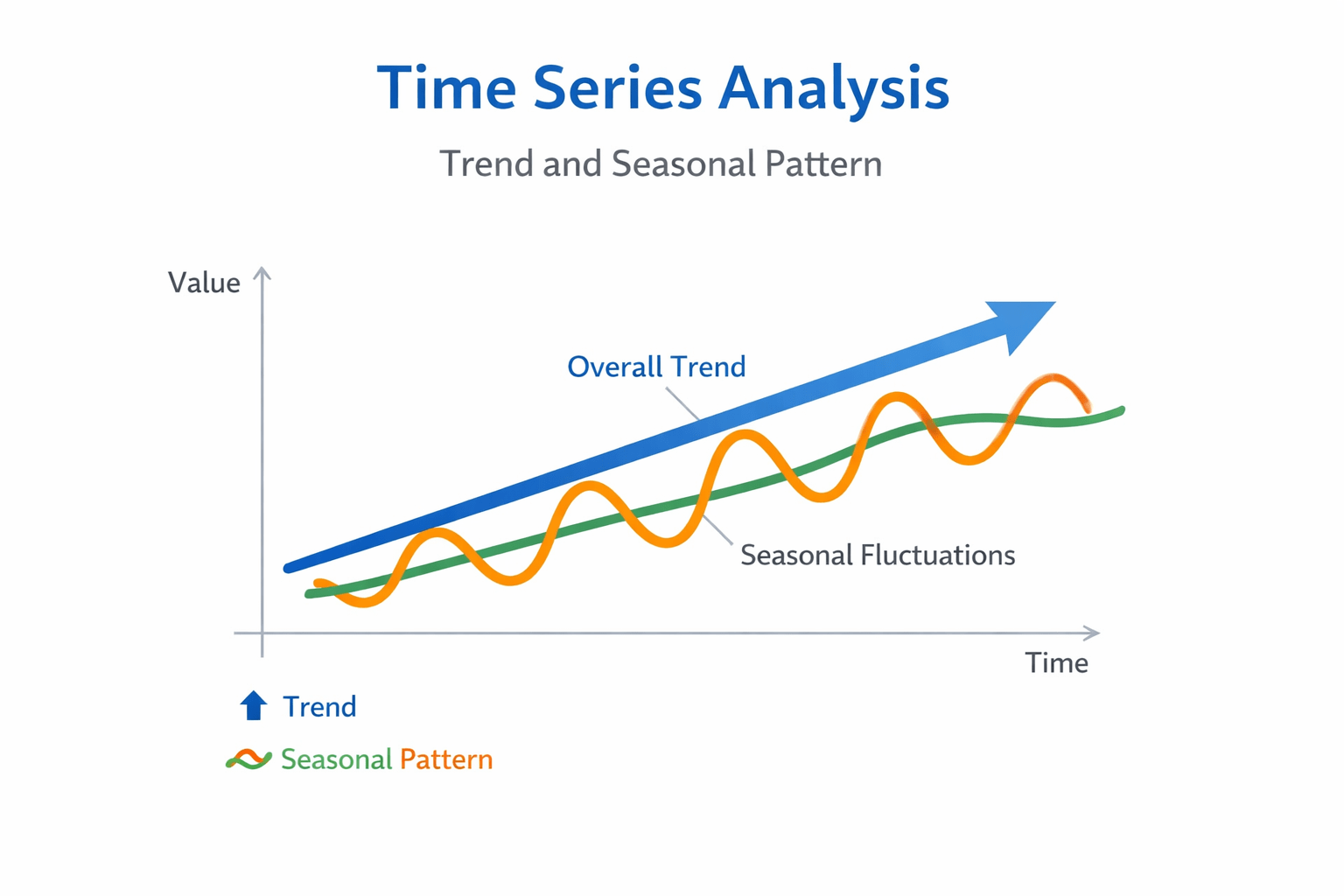
Trend patterns in data
Seasonal patterns
Why data changes over time
Basic forecasting idea
How do we separate these effects?
.
This is where ETS Decomposition helps.
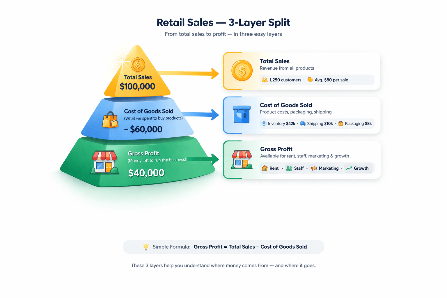
Imagine a retail store analyzing monthly sales
Sales change because of:
Festival seasons
Long-term growth
Random events (weather, economy)
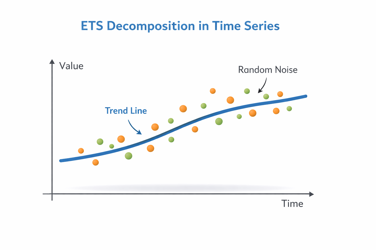
To understand sales patterns we must break the data into components.
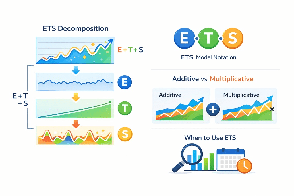
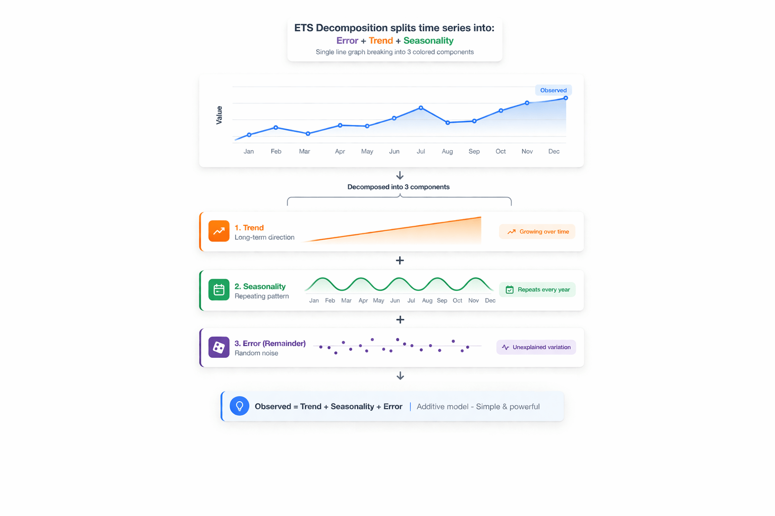
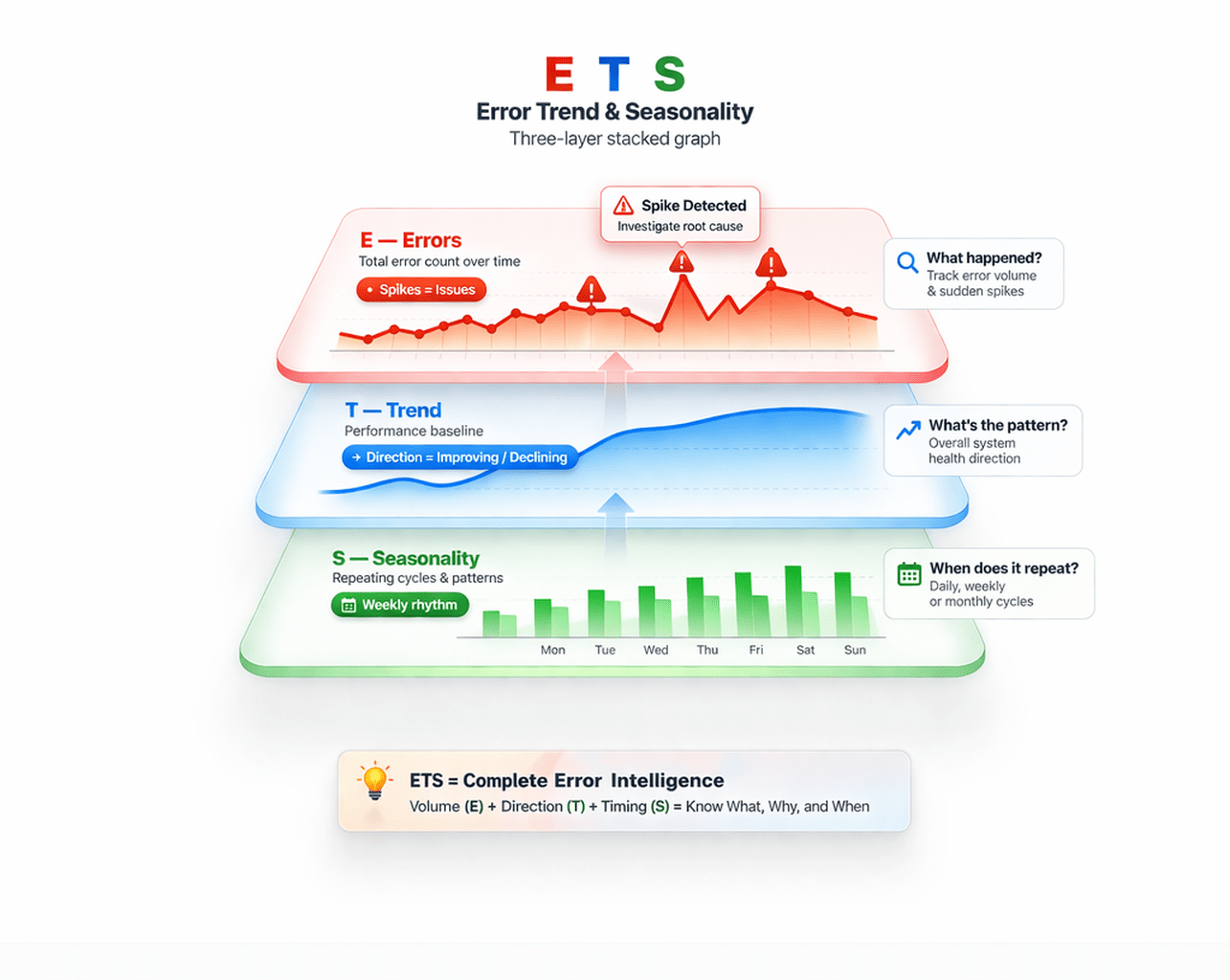
ETS decomposition splits time series into:
Error + Trend + Seasonality
This helps us analyze and forecast data better.
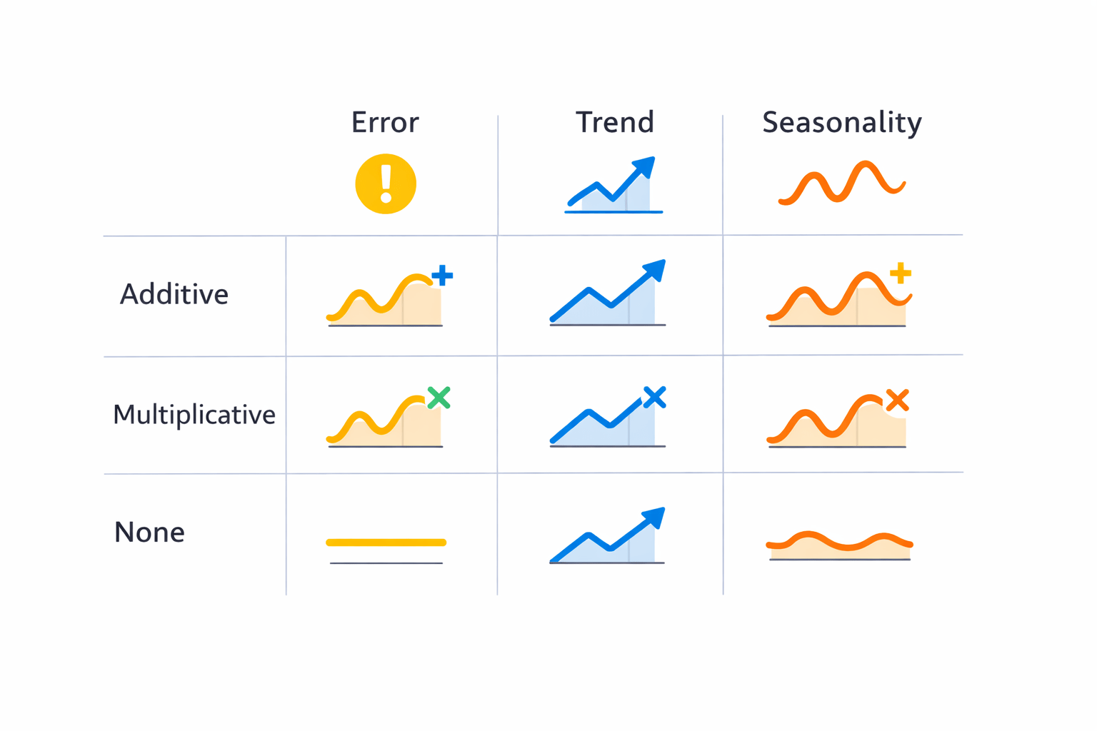
ETS stands for:
E → Error
T → Trend
S → Seasonality
It is a statistical technique to analyze time series structure.
Used in:
Error represents:
Types:
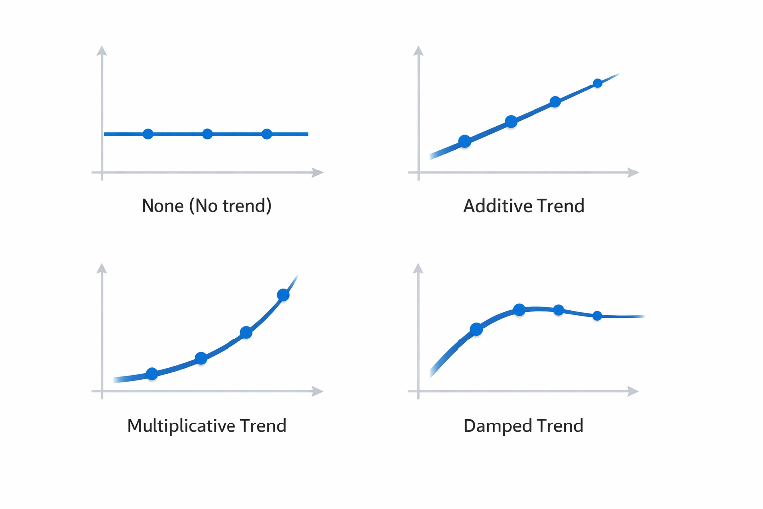
Long-term direction of data
Types:
• None (No trend)
• Additive trend
• Multiplicative trend
• Damped trend
Trend
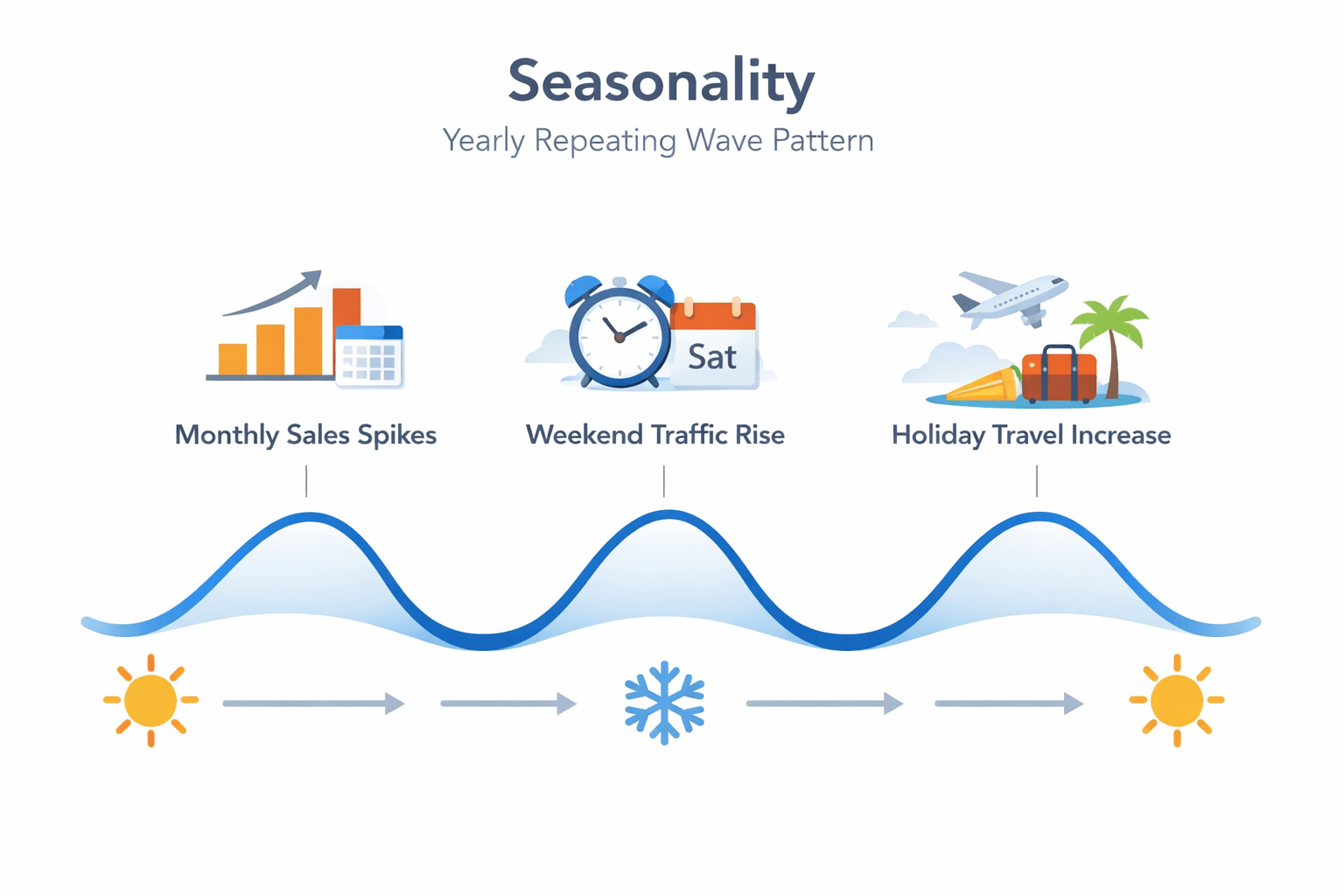
Repeating pattern over fixed time period
Examples:
• Monthly sales spikes
• Weekend traffic rise
• Holiday travel increase
Types:
ETS models follow format: ETS(Error, Trend, Seasonality)
Examples:
ETS(A,N,N)
ETS(M,A,M)
ETS(A,Ad,N)
Each letter defines model behavior.
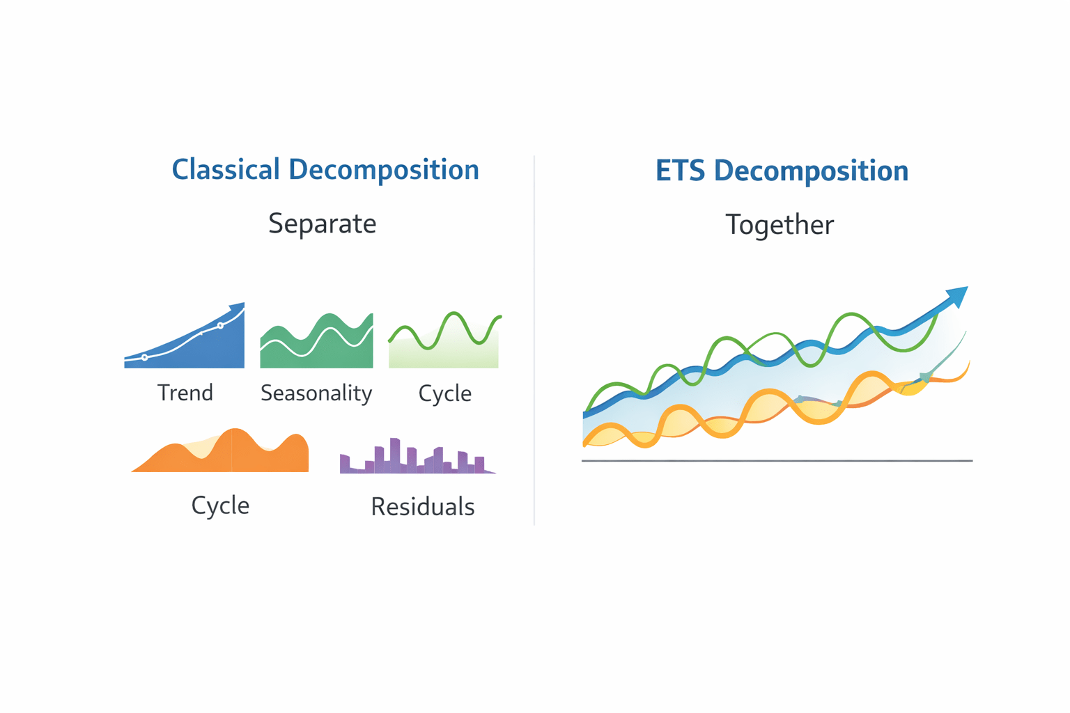
Key difference:
Classical Decomposition
• Components extracted first
ETS Decomposition
• Components modeled together
ETS is more flexible and better for forecasting
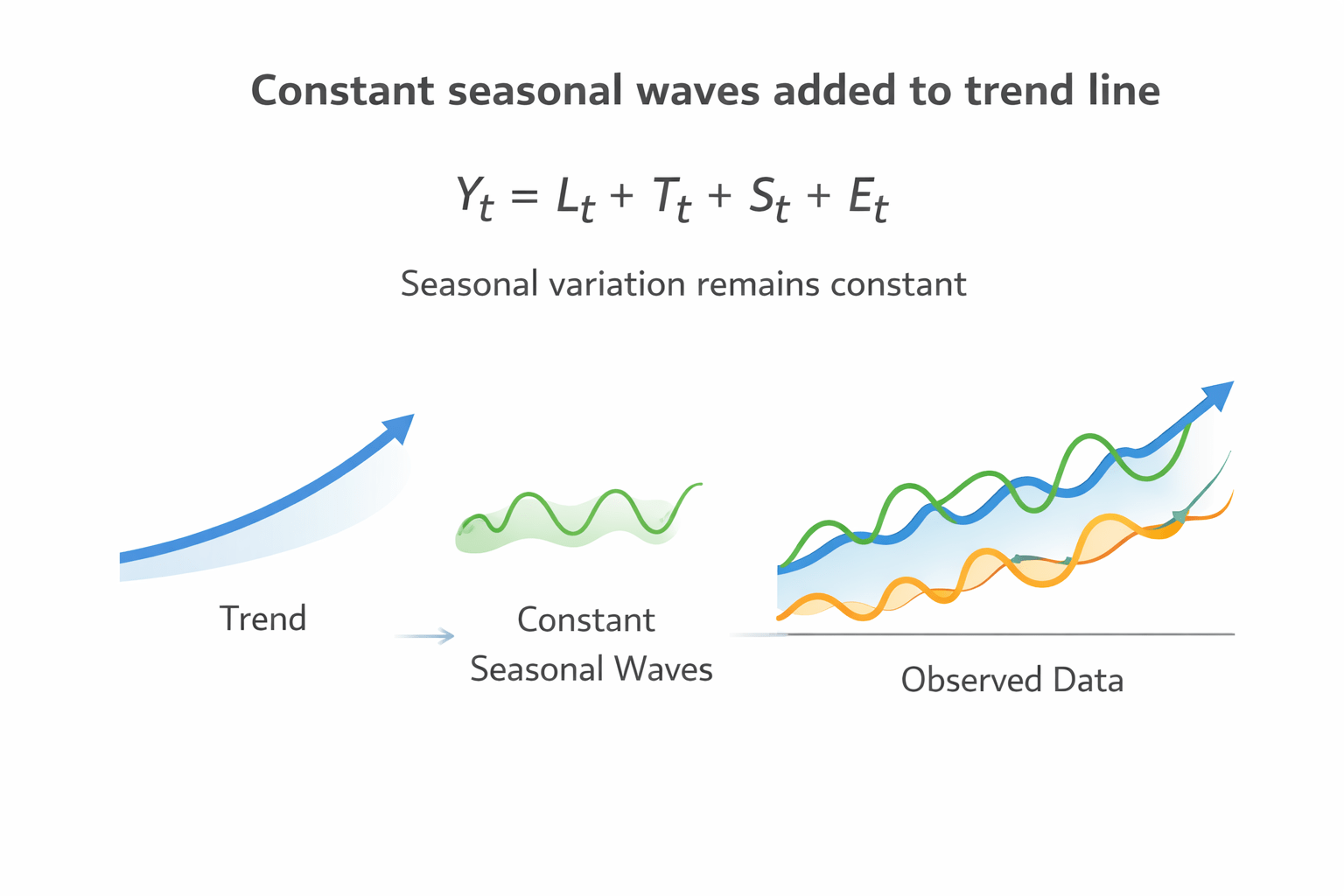
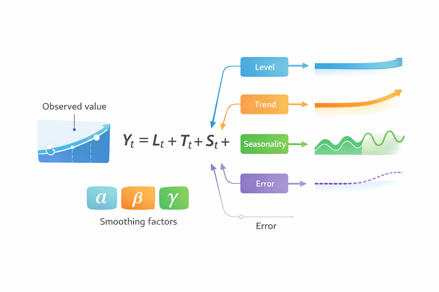
Additive model equation:
Yt = Lt + Tt + St + Et
Used when:
Seasonal variation remains constant
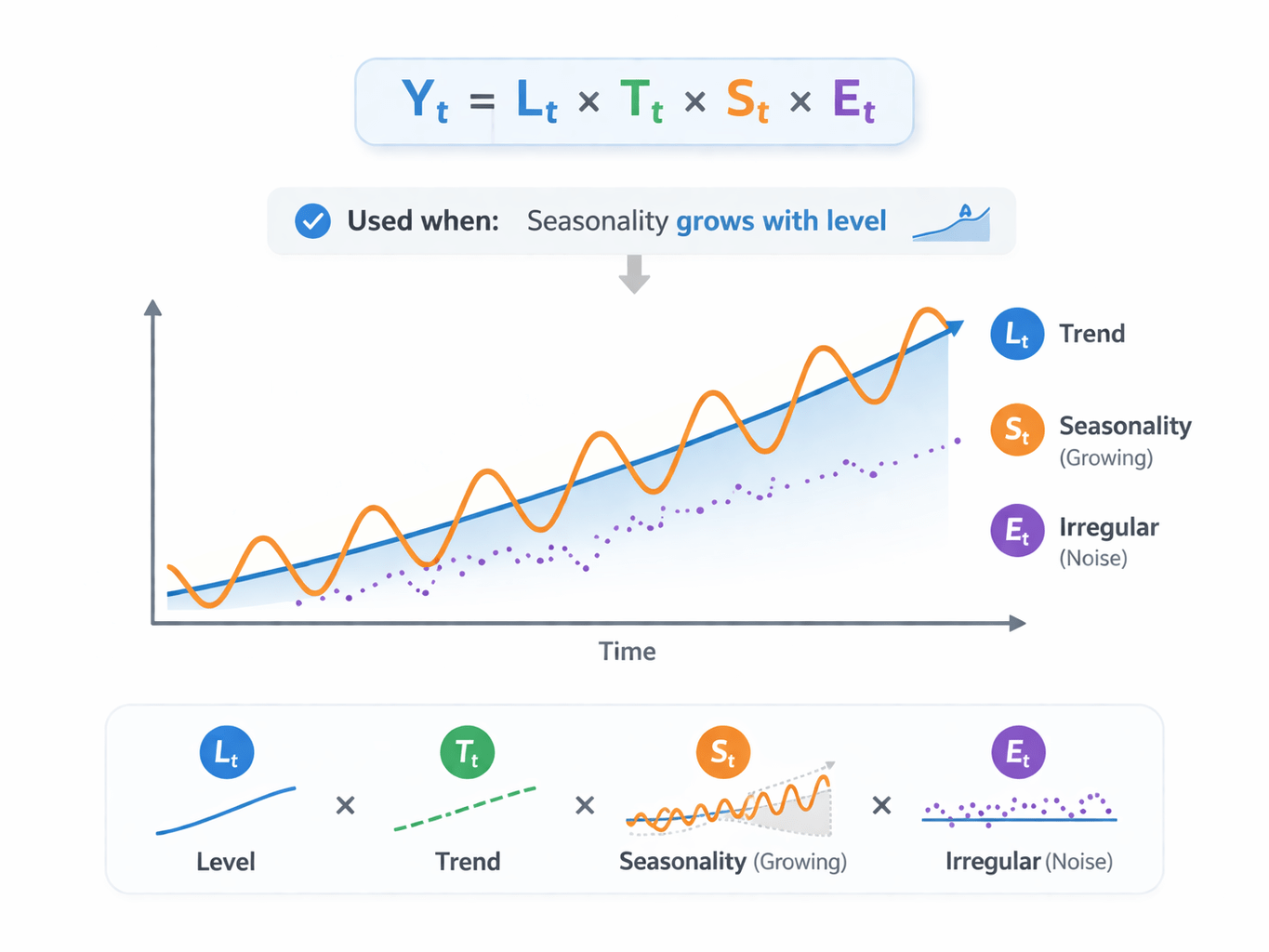
Multiplicative model equation:
Yt = Lt × Tt × St × Et
Used when:
Seasonality grows with level
Important symbols:
Yt → Observed value
Lt → Level
Tt → Trend
St → Seasonality
Et → Error
Parameters:
α β γ → smoothing factors
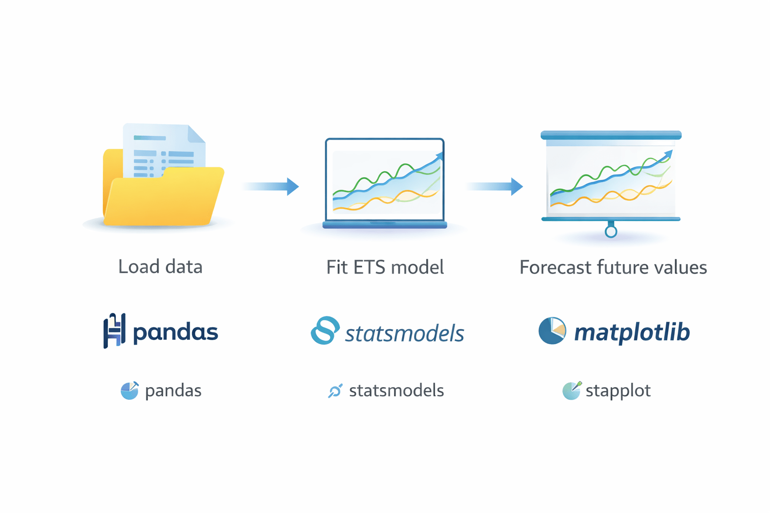
Libraries used:
• pandas
• matplotlib
• statsmodels
Steps:
1 Load data
2 Fit ETS model
3 Forecast future values
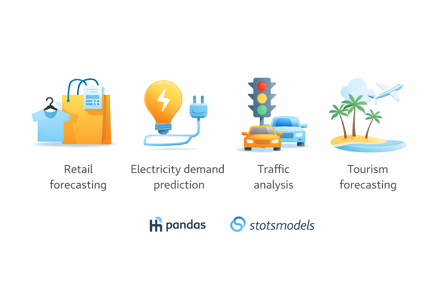
ETS is used in:
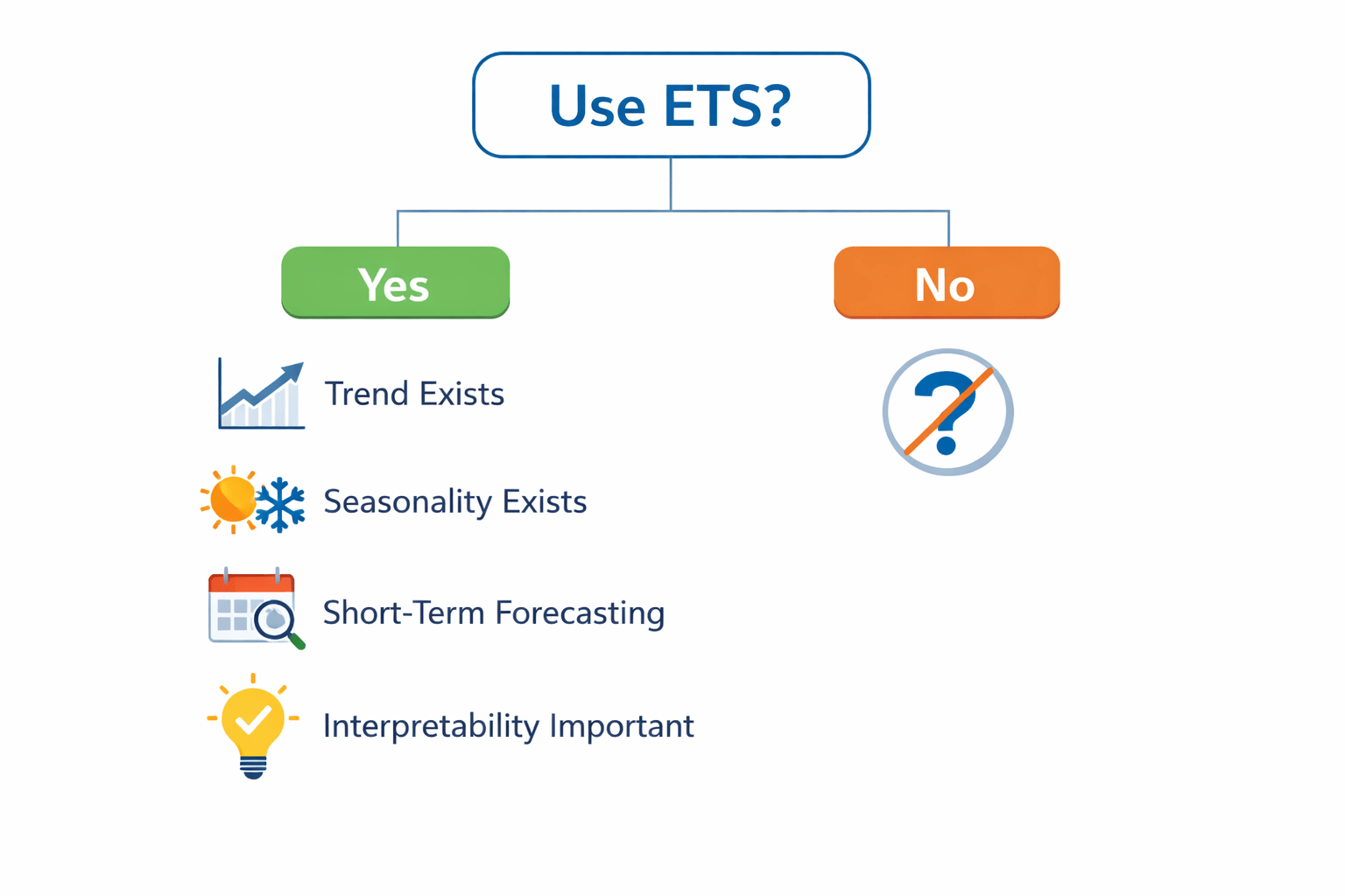
Use ETS when:
• Trend exists
• Seasonality exists
• Short-term forecasting needed
• Interpretability is important

Summary
5
Widely used in business and demand prediction
4
Provides flexible forecasting capability
3
Supports additive and multiplicative models
2
Helps understand data structure clearly
1
ETS splits time series into Error, Trend, Seasonality
Quiz
A dataset shows increasing seasonal variation with sales growth.
Which model type should be used?
A. Additive Seasonality
B. Multiplicative Seasonality
C. No Seasonality
D. Damped Trend
Quiz
A dataset shows increasing seasonal variation with sales growth.
Which model type should be used?
A. Additive Seasonality
B. Multiplicative Seasonality
C. No Seasonality
D. Damped Trend
By Content ITV


