Book 4. Valuation and Risk Models

FRM Part 1

VRM 15. The Black-Scholes Merton Model

Presented by: Sudhanshu

Module 1. Stock Price and Return Distributions

Module 2. Black-Scholes-Merton Model

Module 3. Dividends, Warrants and Implied Volatility

Module 1. Stock Price and Return Distributions

Topic 1. Distribution of Stock Prices and Returns

Topic 2. Expected value

Topic 3. Estimating Historical Volatility

Topic 1. Distribution of Stock Prices and Returns

Lognormal Property of Stock Prices
- The Black-Scholes-Merton (BSM) option pricing model assumes that stock prices are lognormally distributed.
- If is normally distributed, then (stock price at time T) has a lognormal distribution.
- Formula:
  - : stock price at time T
  - : stock price at time 0
  - $μ$ : expected return on stock per year
  - $σ$ : volatility of the stock price per year
  - $N [m, s]$ : normal distribution with mean $m$ and standard deviation $s$
Distribution of Rates of Return
- The BSM model assumes stock returns are normally distributed.
- Mean of Continuously Compounded Returns:
- Standard Deviation of Continuously Compounded Returns:
- Volatility will be lower for longer time periods based on the standard deviation formula.

\ln S_{T}

S_{T}

S_{0}

\ln S_{T} \sim \text{~} N \left[ \ln S_{0} +\left( \mu -\frac{\sigma^{2}}{2}\right)T, \sigma \sqrt{T}\right]

(\mu-\sigma^2/2)

\sigma/\sqrt{T}

Practice Questions: Q1

Q1. XYZ stock has a current price of $30 and an expected value in nine months of $34. The expected annual return is closest to:

A. 11.76%.

B. 12.52%.

C. 13.33%.

D. 16.69%.

Practice Questions: Q1 Answer

Explanation: D is correct.

With a current price of $30, a future price of $34, and a time period of nine months, the formula setup is as follows:
By dividing $34 by $30 and then taking the natural log of both sides, we can solve for μ (the expected rate of return): μ = 0.1669, or 16.69%

\$30 \times e^{\mu 0.75}=\$34.

Q2. Assuming a portfolio has the following asset returns: 6%, 2%, 8%, –3%, what is the realized portfolio return?

A. 3.16%.

B. 3.25%.

C. 4.72%.
D. 4.75%.

Practice Questions: Q2

Explanation: A is correct.

Practice Questions: Q2 Answer

\text{Realized portfolio return }=(1.06 \times 1.02 \times 1.08 \times 0.97)^{1/4}-1=3.16\%

Topic 2. Expected Value

Expected Value of Stock Price :
- : expected rate of return
Example: A stock currently priced at $25 with an expected annual return of 20%. The expected value of the stock in six months is

Realized Return for a Portfolio: When computing the realized return for a portfolio, chain-link the returns.
- Example: For returns of 5%, -4%, 9%, 6%, the realized portfolio return is

(E(S_{T}))

E(S_{T})=S_{0} e^{\mu T}

\mu

25\times e^{0.2 \times 0.5}=\$27.63

(1.05 \times 0.96 \times 1.09 \times 1.06)^{1/4}-1=3.9\%

Topic 3. Estimated Historical Volatility

Scaling Volatility: Volatility for short time periods can be scaled to longer time periods by multiplying by the square root of the number of periods.
- Example: If weekly standard deviation is 5%, annual standard deviation is

Volatility Estimation Process:
- Collect daily price data.
- Compute the standard deviation of the series of corresponding continuously compounded returns.
- Continuously compounded returns can be calculated as .
- Annualized volatility is the estimated volatility multiplied by the square root of the number of trading days in a year.
Data Period: 90-180 trading days of data is often sufficient, but a common rule of thumb is to use data covering a period equal to the projection period (e.g., a year's historical data for a year's volatility estimate).
Impact of Dividends:
- Stock prices naturally decline on the ex-dividend date.
- When calculating historical volatility, the best approach is to remove stock price changes on ex-dividend dates from the dataset

5\% \times \sqrt{52}=36.06\%

\ln(S_{i}/ S_{i-1})

Module 2. Black-Scholes-Merton Model

Topic 1. Assumption of The Black-Scholes-Merton Option Pricing Model

Topic 2. Black-Scholes-Merton Formulas

Topic 1. Assumption of The Black-Scholes-Merton Option Pricing Model

The BSM model values options in continuous time and is based on a no-arbitrage assumption. The key assumptions are:
- The price of the underlying asset follows a lognormal distribution. This means the continuous returns are normally distributed.
- The (continuous) risk-free rate is constant, known, and always available for borrowing or lending.
- Trading is continuous.
- The volatility of the underlying asset is constant and known.
- Markets are "frictionless," meaning no taxes, transaction costs, or restrictions on short sales or their proceeds.
- The underlying asset has no cash flow, such as dividends or coupon payments.
- The options valued are European options, which can only be exercised at maturity. The model does not correctly price American options.

Practice Questions: Q3

Q3. Which of the following is not an assumption underlying the BSM options pricing model?

A. The underlying asset does not generate cash flows.

B. Continuously compounded returns are lognormally distributed.

C. The option can only be exercised at maturity.

D. The risk-free rate is constant.

Practice Questions: Q3 Answer

Explanation: B is correct.

Assumptions underlying the BSM options pricing model include the following:

Asset price (not returns) follows a lognormal distribution.
The (continuous) risk-free rate is constant.
Trading is continuous.
The volatility of the underlying asset is constant.
Markets are frictionless.
The asset has no cash lows.
The options are European (i.e., they can only be exercised at maturity).

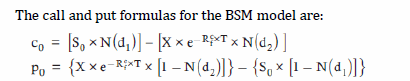
Topic 2. Black-Scholes-Merton Formulas

Call Option Formula
Put Option Formula

Where:

$T =$ time to maturity (as % of a 365-day year)
$=$ asset price
$X =$ exercise price
$=$ continuously compounded risk-free rate
$σ =$ volatility of continuously compounded returns on the stock
$N (\cdot) =$ cumulative normal probability
Put-Call Parity: If one option price is known, the other can be calculated using put-call parity (with continuously compounded interest rates).

(c_0): c_{0}=[S_{0} \times N(d_1)]-[X \times e^{-R_f^c \times T} \times N(d_2)]

{p}_0=\left\{X \times e^{-R_f^e \times T} \times\left[1-N\left(d_2\right)\right]\right\}-\left\{S_0 \times\left[1-N\left(d_1\right)\right]\right\}

({p}_0);

d_1=\frac{\ln \left(\frac{S_0}{X}\right)+\left[R_f^e+\left(0.5 \times \sigma^2\right)\right] \times T}{\sigma \times \sqrt{T}}

d_2=d_1-(\sigma \times \sqrt{T})

S_0

R_f^c

c_0=p_0+S_0-\left(X \times e^{-R_f^\epsilon \times T}\right)

p_0=c_0-S_0+\left(X \times e^{-R_f^\epsilon \times T}\right)

Practice Questions: Q4

Q4. A European put option has the following characteristics: = $50; X = $45; r = 5%; T = 1 year; and σ = 25%. Which of the following is closest to the value of the put?

A. $1.88.

B. $3.28.

C. $9.06.

D. $10.39.

S_0

Practice Questions: Q4 Answer

Explanation: A is correct.

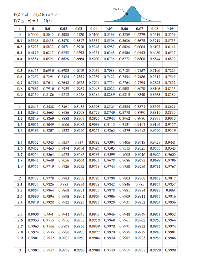
From the cumulative normal table:

\begin{aligned} & S_0=\$ 50 ; X=\$ 45 ; r=5 \% ; T=1 \text { year; and } \sigma=25 \% \\ & d_1=\frac{\ln \left(\frac{50}{45}\right)+\left(0.05+\frac{0.0625}{2}\right) 1}{0.25(1)}=\frac{0.18661}{0.25}=0.74644 \\ & d_2=0.74644-0.25=0.49644 \end{aligned}

\begin{aligned}N(–d_1)& = 0.2266\\ N(–d_2)& = 0.3085^{\text{*}}\\ p &=45 e^{-0.05(1)}(0.3085)-50(0.2266)=1.88\end{aligned}

Practice Questions: Q5

Q5. A European call opotin has the following characteristics: = $50; X = $45; r = 5%; T = 1 year; and σ = 25%. Which of the following is closest to the value of the call?

A. $1.88.

B. $3.28.

C. $9.06.

D. $10.39.

S_0

Practice Questions: Q5 Answer

Explanation: C is correct.

from the cumulative normal table:

\begin{aligned} & \mathrm{S}_0=\$ 50 ; \mathrm{X}=\$ 45 ; \mathrm{r}=5 \% ; \mathrm{T}=1 \text { year; and } \sigma=25 \% \\ & \mathrm{~d}_1=\frac{\ln \left(\frac{50}{45}\right)+\left(0.05+\frac{0.0625}{2}\right) 1}{0.25(1)}=\frac{0.18661}{0.25}=0.74644 \\ & \mathrm{~d}_2=0.74644-0.25=0.49644 \end{aligned}

\begin{aligned} & \mathrm{N}\left(\mathrm{~d}_1\right)=0.7731 \\ & \mathrm{~N}\left(\mathrm{~d}_2\right)=0.6915^* \\ & \mathrm{c}=50(0.7731)-45 \mathrm{e}^{-0.05}(0.6915)=9.055 \end{aligned}

Practice Questions: Q6

Q6. A security sells for $40. A 3-month call with a strike of $42 has a premium of $2.49. The risk-free rate is 3%. What is the value of the put according to put-call parity?

A. $1.89.

B. $3.45.

C. $4.18.

D. $6.03.

Practice Questions: Q6 Answer

Explanation: C is correct.

\mathrm{p}=\mathrm{c}+\mathrm{Xe}^{-\mathrm{rT}}-\mathrm{S}=2.49+42 \mathrm{e}^{-0.03 \times 0.25}-40=\$ 4.18

Practice Questions: Q7

Q7. Stock ABC trades for $60 and has 1-year call and put opotins written on it with an exercise price of $60. The annual standard deviation estimate is 10%, and the continuously compounded risk-free rate is 5%. The value of both the call and put using the BSM option pricing model are closest to which of the following?

A. Call: $6.21; Put: $1.16

B. Call: $4.09; Put: $3.28

C. Call: $4.09; Put: $1.16

D. Call: $6.21; Put: $3.28

Practice Questions: Q7 Answer

Explanation: C is correct.

First, let’s compute and as follows:

Now, look up these values in the normal table at the back of this book. These values are and . Hence, the value of the call is:

According to put-call parity, the put’s value is:

d_1

d_2

N(d_1)=0.7088

N(d_2)=0.6736

\begin{aligned} & \mathrm{d}_1=\frac{\ln \left(\frac{60}{60}\right)+\left[0.05+\left(0.5 \times 0.10^2\right)\right] \times 1.0}{0.1 \times \sqrt{1.0}}=0.55 \\ & \mathrm{~d}_2=0.55-(0.1 \times \sqrt{1.0})=0.45 \end{aligned}

\begin{aligned} c_0 & =\$ 60(0.7088)-\left[\$ 60 \times \mathrm{e}^{-(0.05 \times 1.0)} \times(0.6736)\right] \\ & =\$ 42.53-\$ 38.44 \\ & =\$ 4.09 \end{aligned}

\begin{aligned} P_0 & =c_0-S_0+\left(X \times \mathrm{e}^{-R \xi \times T}\right) \\ & =\$ 4.09-\$ 60.00+\left[\$ 60.00 \times \mathrm{e}^{-(0.05 \times 1.0)}\right] \\ & =\$ 1.16 \end{aligned}

Module 3. Dividends, Warrants, And Implied Volatility

Topic 1. Valuation of European Options

Topic 2. Impact of Dividends on American Options

Topic 3. Valuation of Warrants

Topic 4. Volatility Estimation

Topic 1. Valuation of European Options

On Non-Dividend-Paying Stock: Calculated directly using the BSM formulas.
On Dividend-Paying Stock:
- The BSM assumption that the underlying asset has no cash flows is relaxed.
- For a continuous dividend yield (q), is substituted for in the BSM formula.
- Cash flows (dividends) increase put values and decrease call values.
- If the dollar amount of dividends is given, compute the present value of the dividends and subtract that amount from the stock price ( ) before
  applying the BSM model.
On Foreign Currencies:
- The foreign risk-free rate ( $r_{f}$ ) is substituted for the continuous dividend yield (q) in the component of the BSM model.
On Futures:
- The stock price ( $S_{0}$ ) in the component is replaced with the futures price (F).
- The dividend yield (q) is replaced with the domestic risk-free rate (r).

S_0 \times e^{-q T}

S_0

S_0 \times e^{-q T}

Practice Questions: Q8

Q8. Assume a current stock price of $35 with a continuously compounded dividend yield of 2.5%. There is a 6-month call option on the stock with an exercise price of $33. What is the adjusted stock price to use for the BSM model?

A. $30.12.

B. $32.59.

C. $34.57.

D. $35.44.

Practice Questions: 8 Answer

Explanation: C is correct.

The adjusted stock price is calculated as:

\text { adjusted stock price }=\$ 35 \times \mathrm{e}^{-0.025 \times 0.5}=\$ 34.57

When no dividends are paid, there is generally no difference in value between European and American call options, as early exercise is not optimal.
American Call Options:
- Dividends complicate the early exercise decision because a dividend payment effectively decreases the stock price.
- Early exercise becomes more optimal the closer the option is to expiration and the larger the dividend.
- An investor will exercise early if
American Put Options:
- Early exercise becomes less likely with larger dividends.
- The value of the put option increases as the dividend is paid.

Topic 2. Impact of Dividends on American Options

D_n > X(1-e^{-r(T-t_n)})

Practice Questions: Q9

Q9. Compared to the value of a call option on a stock with no dividends, a call option on an identical stock expected to pay a dividend during the term of the option will have a:

A. lower value in all cases.

B. higher value in all cases.

C. lower value only if it is an American-style option.

D. higher value only if it is an American-style option

Practice Questions: Q9 Answer

Explanation: A is correct.

An expected dividend during the term of an option will decrease the value of a call option.

Topic 3. Valuation of Warrants

Description: Warrants are attachments to a bond issue that grant the holder the right to purchase shares of a security at a stated price.
Valuation: Warrants can be valued as a separate call option on the firm’s shares.
- Unlike call options where shares are already outstanding, exercising warrants involves purchasing shares directly from the firm.
- This can affect the value of all outstanding shares, leading to dilution of equity per share.
Dilution Cost to Existing Shareholders:
- Assuming no benefit to the company from issuing warrants, the value of each warrant is computed by adjusting the regular call option value for dilution.
- Formula: Value of each warrant value of regular call option
  - $N$ : number of shares outstanding
  - $M$ : number of new warrants issued
- The company’s stock price is expected to decline by:

=\frac{N}{N+M} \times

\frac{M}{N+M} \times \text {value of regular call option}.

Practice Questions: Q10

Q10. There are 3 million outstanding shares of ABC stock currently selling at $42 each. ABC is considering issuing 1 million warrants with a strike price of $45 exercisable in one year. If the current value of a 1-year European call option is $2.12, the expected stock price after announcing the warrant (assuming no perceived benefit to issuance) will be closest to:

A. $40.41.

B. $41.47.

C. $42.53.

D. $43.59.

Practice Questions: Q10 Answer

Explanation: B is correct.

The value of each warrant is equal to:

The total warrant cost is 1,000,000 × $1.59 = $1.59 million.
The initial stock price will therefore decline by:

So, the stock price = $42.00 – $0.53 = $41.47.

\frac{3,000,000}{3,000,000+1,000,000} \times \$ 2.12=\$ 1.59

\frac{1,000,000}{3,000,000+1,000,000} \times \$ 2.12=\$ 0.53

Implied Volatility: Volatility is generally unobservable in the BSM call and put equations.
- Implied volatility is the value for the standard deviation of continuously compounded rates of return that is implied by the market price of the option.
- It is calculated by using the BSM option pricing model along with market prices for options and solving for volatility.
- There is no closed-form solution; it must be found by iteration (trial and error).
- If the BSM-calculated call value is lower than the market price, volatility needs to be increased (and vice versa) until the model value equals the market price, as option value and volatility are positively related.
Historical Volatility: Historical volatility is the standard deviation of a past series of continuously compounded returns for the underlying asset.
- It can serve as a basis for future volatility but may not always represent the current market.
- Steps for computation include converting prices to returns, then to continuously compounded returns, and then calculating the variance and standard deviation.

Topic 4. Volatility Estimation

Practice Questions: Q11

Q11. Which of the following statements is most accurate regarding implied volatility in the BSM model?

A. Volatility is constant across strike prices.

B. Volatility is most accurately applied using historical data.

C. The process for estimating volatility involves two steps at most.

D. Volatility is often derived using the BSM market price and the other inputs.

Practice Questions: Q11 Answer

Explanation: D is correct.

Volatility is not directly observable, and so to estimate it, the price of the option using the BSM model and the other observable inputs (stock price, exercise price, risk-free rate, and time to maturity) are put into the model to derive volatility. Volatility is not constant across strike prices. Using historical data to estimate volatility is helpful, but it does not predict current or future volatility. The
process for estimating volatility requires many steps, as it is a trial-and-error process.