Book 4. Valuation and Risk Models
FRM Part 1
VRM 14. Binomial Trees
Presented by: Sudhanshu
Module 1. One-Step Binomial Model
Module 2. Two-Step Binomial Model and Model Modifications
Module 1. One-Step Binomial Model

Topic 1. Introduction to One-Step Model
Topic 2. Example of a One-Step Model
Topic 3. Risk-Neutral Valuation
Topic 4. Risk-Neutral Valuation Example
Topic 5. Using Delta to Develop a Replicating Portfolio
Topic 1. Introduction to One-Step Model
-
Assumes stock can move to only two prices over one time period:
-
Up state:
-
Down state:
-
- Simplifies option pricing by assuming discrete outcomes
-
Key variables:
- P: Current stock price
- XXX: Strike price
- ttt: Time to expiration
- rrr: Risk-free rate (continuously compounded)
- u,du, du, d: Up/down factors
-
Useful for:
- Understanding foundational pricing concepts
- Introducing replication and hedging logic
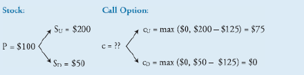
Topic 2. Example of a One-Step Model
-
Example Input:
-
-
-
- Construct a hedged portfolio: Long shares and short 1 call option
-
Solve for Δ\Delta
- In up state:
- In down state:
-
Set both equal:
-
- Portfolio value in one year:
- Solve for call price:
50Δ50\Delta
Topic 3. Risk-Neutral Valuation
-
Based on no-arbitrage and law of one price
-
Law of one price: If two investments provide the same cash flows at
the same times in the future, they both should sell for exactly the same price.
-
Investors assume risk-neutral valuation:
-
Expected return = risk-free rate
-
-
Up/down factors:
-
Risk-neutral probability:
-
Option value:
-
- Used in both one- and multi-step binomial models
Topic 4. Risk-Neutral Valuation Example
-
Given:
-
- Payoffs:
- Expected value in 1 year:
- Discounted call price:
Practice Questions: Q1
Q1. Suppose a 1-year European call option exists on XYZ stock. The current continuously compounded risk-free rate is 3% and XYZ does not pay a dividend. Assume an annual standard deviation of 8%.
The risk-neutral probability of an up move for the XYZ call option is:
A. 0.31.
B. 0.69.
C. 0.92.
D. 1.08.
Practice Questions: Q1 Answer
Explanation: B is correct.
First, calculate the size of the up- and down-move factors:
The risk-neutral probability of an up move is then calculated as:
Topic 5. Using Delta to Develop a Replicating Portfolio
-
Hedging: Eliminating price variation by short selling an asset with same price volatility as the asset being hedged.
-
Hedge Ratio: Number of asset units needed to completely eliminate the price volatility of one call option.
-
Delta ( ) = Sensitivity of option value to stock movement
-
Formula:
-
Replicating portfolio:
-
Long shares, short 1 option → hedge risk
-
-
Example:
-
Practice Questions: Q2
Q2. An investor is analyzing a 1-year European call option with an exercise price of $18. The stock value in the up state is $30, while the value in the down state is $10. The delta for this option is closest to:
A. 0.40.
B. 0.60.
C. 0.67.
D. 0.90.
Practice Questions: Q2 Answer
Explanation: B is correct.
Delta provides the number of units of stock to hold per call option to be shorted to implement a hedge. If the stock price goes up to $30, the call option with an exercise price of $18 will be worth $12. If the stock price goes down to $0, the call option will be worth $0.
Module 2. Two-Step Binomial Model and Model Modifications
Topic 1. Introduction to Two-Step Model
Topic 2. Modifying the Binomial Model
Topic 3. American Options
Topic 4. Increasing the Number of Time Periods
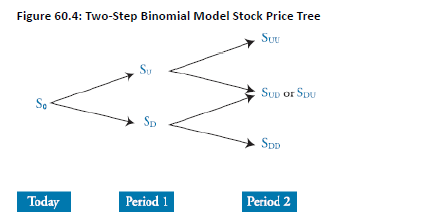
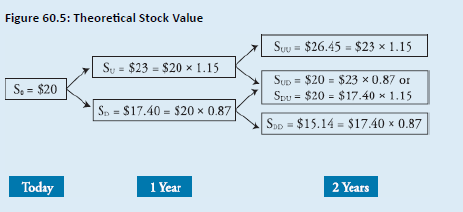
Topic 1. Introduction to Two-Step Model
-
Extends tree by adding second time step
-
More realistic: allows more outcomes
- Paths: Up-Up, Up-Down, Down-Up, Down-Down
-
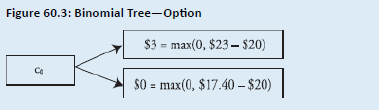
Terminal node payoffs computed first
-
Value is back-calculated using risk-neutral probabilities
-
Key formula:
-
-
- Used for pricing both European and American options
-
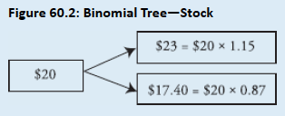
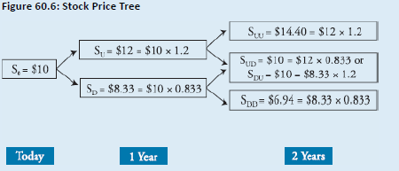
Same stock:
-
Nodes:
-
Payoffs:
-
Backward induction:
- Compute expected value at each node
- Discount back to time 0
- Final option value ≈ discounted expected value from tree
Topic 1. Introduction to Two-Step Model
Practice Questions: Q3
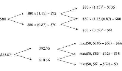
Q3. Assume the stock price is currently $80, the stock price annual up-move factor is 1.15, and the riskfree rate is 3.9%. The value of a 2-year European call option with an exercise price of $62 using a
two-step binomial model is closest to:
A. $0.00.
B. $18.00.
C. $23.07.
D. $24.92.
Practice Questions: Q3 Answer
Explanation: C is correct.
Practice Questions: Q4
Q4. Assume the stock price is currently $80, the stock price annual up-move factor is 1.15, and the riskfree rate is 3.9%. The value of a 2-year European put option with an exercise price of $62 using a
two-step binomial model is closest to:
A. $0.42.
B. $16.89.
C. $18.65.
D. $21.05.
Practice Questions: Q4 Answer
Explanation: A is correct. Using put-call parity
-
The binomial model is adaptable to different underlying assets by modifying the risk-neutral probability formula:
-
Dividend-Paying Stocks / Indices:
- Let qqq be the continuous dividend yield
- Adjusted risk-neutral probability:
- Total return = dividend + capital gain → lower capital gain than non-dividend stocks
-
Currency Options: Let
-
Adjusted formula:
- Reflects return earned on foreign-denominated assets
-
Adjusted formula:
-
Futures Options: Futures require no initial investment. Modify risk-neutral formula:
-
- These changes ensure accurate pricing for assets with dividends, interest rate differentials, or zero-cost entry.
Topic 2. Modifying the Binomial Model
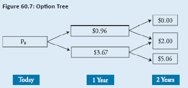
Topic 3. American Options
- American options can be exercised at any time → must evaluate early exercise at every node.
- Valuation:
- Example:
-
At Year 1 down-node:
- Intrinsic Value= 3.67 and Continuation Value = 3.43. Since 3.67 > 3.43 → Exercise is Optimal
- American calls on non-dividend stocks are never exercised early
- Early exercise more relevant for puts and dividend-paying stocks
Practice Questions: Q5
Q5. A 1-year American put option with an exercise price of $50 will be worth either $8 at maturity with a probability of 0.45 or $0 with a probability of 0.55. The current stock price is $45. The risk-free
rate is 3%. The optimal strategy is to:
A. exercise the option because the payoff from exercise exceeds the present value of the expected future payoff.
B. not exercise the option because the payoff from exercise is less than the discounted present value of the future payoff.
C. exercise the option because it is currently in the money.
D. not exercise the option because it is currently out of the money.
Practice Questions: Q5 Answer
Explanation: A is correct.
The payoff from exercising the option is the exercise price minus the current stock price: $50 – $45 = $5. The discounted value of the expected future payoff is:
It is optimal to exercise the option early because it is worth more exercised ($5.00) than if not exercised ($3.49).
Practice Questions: Q6
Q6. The annual standard deviation for Baker stock is 11%. The continuously compounded risk-free rate is 3.5% per year, and Baker pays dividends at a yield of 2%. The risk-neutral probability of a
downward move is closest to:
A. 0.366.
B. 0.459.
C. 0.541.
D. 0.634
Practice Questions: Q6 Answer
Explanation: B is correct.
There are several steps needed for this calculation. The first is to calculate U (the size of the up-move factor), which is equal to Therefore, D (the size of the down-move factor) is 1/ 1.116278, or 0.895834. Next, the risk-neutral probability of an upward move is calculated as:
Finally, the risk-neutral probability of a downward move is calculated as:
Topic 4. Increasing the Number of Time Periods
-
More time steps = finer approximation of continuous price paths.
-
As step size Δt→0\Delta t \to 0 , binomial model converges to the Black-Scholes-Merton (BSM) model.
-
Increased steps → more nodes → better realism in pricing
-
Allows better modeling of:
-
Path-dependency
-
Early exercise (American options)
- High volatility effects
-
-
Mathematical Convergence:
-
Practical Use:
- Real-world applications use 100–1,000+ time steps for accuracy.
- Trade-off: More precision vs. more computation
limΔt→0Binomial Value=BSM Value\lim_{\Delta t \to 0} \text{Binomial Value} = \text{BSM Value}
Practice Questions: Q7
Q7. Using a binomial model, the price of a call option is equal to $3.46. For the same option, the Black- Scholes-Merton model produces a price of $3.38. If the time intervals used in the binomial model are shortened, the expectation is that:
A. $3.38 will get closer to $3.46.
B. $3.46 will get closer to $3.38.
C. the price for both models will be approximately $3.42.
D. there will be no change in the gap between prices.
Practice Questions: Q7 Answer
Explanation: B is correct.
As time intervals are shortened, the price produced by the binomial model will converge toward the Black-Scholes-Merton model price. In this case, the $3.46 price will get lower until it eventually lands at $3.38.