Book 2. Quantitative Analysis
FRM Part 1
QA 4. Multivariate Random Variables
Presented by: Sudhanshu
Module 1. Marginal And Conditional Distributions For Bivariate Distributions
Module 2. Moments Of Bivariate Random Distributions
Module 3. Behavior Of moments For Bivariate Random Variables
Module 4. Independent And Identically Distributed Random Variables
Module 1. Marginal And Conditional Distributions For Bivariate Distributions

Topic 1. Probability Matrix
Topic 2. Marginal and Conditional Distributions
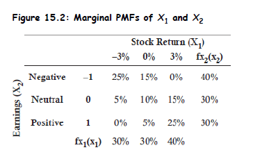
Topic 1. Probability Matrix
- Definition: A probability matrix visually expresses the joint probability mass function (PMF) of discrete random variables - say, stock return and an earnings signal .
-
Why useful?
- Helps model dependencies between variables.
- Critical in understanding joint behavior in finance - e.g., return vs. macro indicators.
-
Key Properties:
- All entries ≥ 0 and ≤ 1.
- Sum of all cells = 1:
Topic 2. Marginal and Conditional Distributions
-
Marginal PMF: Gives the distribution of one variable, summing out the other:
-
-
Conditional PMF: Probability of one variable given the other
-
-
Example: Given earnings = negative ( = –1, total prob = 0.40):
Practice Questions: Q1
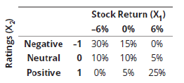
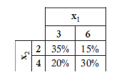
Q1. Suppose a hedge fund manager expects a stock to have three possible returns (–6%, 0%,6%) following negative, neutral, or positive changes in analyst ratings, respectively. The fund manager constructs the following bivariate probability matrix for the stock.
What is the marginal probability that the stock has a positive analyst rating?
A. 10%.
B. 15%.
C. 25%.
D. 30%.
Practice Questions: Q1 Answer
Explanation: D is correct.
The marginal distribution for a positive analyst rating is computed by summing the third row consisting of all possible outcomes of a positive rating as follows:
Practice Questions: Q2
Q2. Suppose a hedge fund manager expects a stock to have three possible returns (–6%, 0%,6%) following negative, neutral, or positive changes in analyst ratings, respectively. The fund manager constructs the following bivariate probability matrix for the stock.
What are the conditional probabilities of the three monthly stock returns given that the analyst rating is positive?
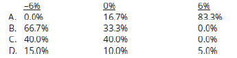
Practice Questions: Q2 Answer
Explanation: A is correct.
A conditional distribution is defined based on the conditional probability for a
bivariate random variable given . All possible outcomes of a positive analyst
rating are found in the third row of the bivariate probability matrix ( ) as
0%, 5%, and 25% for monthly returns of –6%, 0%, and 6%, respectively. These
joint probabilities are then divided by the marginal probability of a positive
analyst rating, which is computed as 0% + 5% + 25% = 30%. Thus, the conditional
distribution for is computed as 0% / 30%, 5% / 30%, and 25% / 30% and
summarized as follows:
Module 2. Moments of Bivariate Random Distributions
Topic 1. Expectation of a Bivariate Random Function
Topic 2. Covariance and Correlation Between Random Variables
Topic 3. Relationship Between Covariance and Correlation
Topic 1. Expectation of a Bivariate Random Function
- Definition: For any function
-
Example: Compute
- Using joint PMF values:
- If returns and earnings are coded numerically (e.g., 3% = 0.03, negative = -1), compute each product, then sum.
- Useful in computing covariance and cross-moments for risk modeling.
Practice Questions: Q3
Q3. What is the expectation of the function using the following joint PMF?
A. 226.4.
B. 358.9.
C. 394.7.
D. 413.6.
Practice Questions: Q3 Answer
Explanation: D is correct.
The expectation is computed as follows:
Topic 2. Covariance and Correlation
- Covariance:
-
Why important?
- Measures linear dependency: how returns and earnings move together.
- Used in portfolio theory, factor models, and risk aggregation.
- Covariance Matrix:
-
Examples:
- Negative Covariance: Stock vs. Put Option
- Zero Covariance: Stock vs. Risk-free asse
Topic 3. Relationship Between Covariance and Correlation
- Correlation standardizes covariance:
- Range:
- Two variables that are independent have a correlation of 0 (i.e., no linear relationship).
-
However, a correlation of 0 does not necessarily imply independence.
- Easy to compare across variable scales
-
Finance context:
- High correlation between asset returns ⇒ poor diversification
- Zero correlation ideal for risk reduction
Practice Questions: Q4
Q4. A hedge fund manager computed the covariances between two bivariate random variables. However, she is having difficulty interpreting the implications of the dependency between the two variables as the scale of the two variables are very different. Which of the following statements will most likely benefit the fund manager when interpreting the dependency for these two bivariate random variables?
A. Compute the correlation by multiplying the covariance of the two variables by the product of the two variables’ standard deviations.
B. Disregard the covariance for bivariate random variables as this data is not
relevant due to the nature of bivariate random variables.
C. Compute the correlation by dividing the covariance of the two variables by the product of the two variables’ standard deviations.
D. Divide the larger scale variables by a common denominator and rerun the estimations of covariance by subtracting each variable’s expected mean.
Practice Questions: Q4 Answer
Explanation: C is correct.
Correlation will standardize the data and remove the difficulty in interpreting the scale difference between variables. Correlation is determined by dividing the covariance of the two variables by the product to the two variables’ standard deviations. The formula for correlation is as follows:
Module 3. Behavior Of Moments For Bivariate Random Variables
Topic 1. Linear Transformations
Topic 2. Variance of Weighted Sum of Bivariate Random Variables
Topic 3. Impact of Correlation on the Standard Deviation
Topic 4. Conditional Expectations
Topic 1. Linear Transformations
- Let
-
Effects: Sign of b determines correlation:
- Variance scales:
- Covariance transforms:
-
Extra Concepts:
- Coskewness and Cokurtosis: Measure higher-order dependencies — used in tail risk modeling
Topic 2. Variance of Weighted Sum of Bivariate Random Variables
- Objective: Measure the total variance of a two-asset portfolio combining two random variables and with weights a and b.
- Formula:
-
Where:
- a: weight of asset 1 in the portfolio
- bbb: weight of asset 2 in the portfolio
- covariance between asset returns
-
Special Case (correlation given instead of covariance):
-
- In a two-asset portfolio:
-
The minimum variance portfolio (i.e., optimal risk weight) is:
-
-
Practice Questions: Q5
Q5. What is the variance of a two-asset portfolio given the following covariance matrix and a correlation between the two assets of 0.25? Assume the weights in Asset 1 and Asset 2 are 40% and 60%, respectively.
A. 0.27%.
B. 0.79%.
C. 1.47%.
D. 2.63%.
Practice Questions: Q5 Answer
Explanation: A is correct.
The variance of this two-asset portfolio is computed as:
Topic 3. Impact of Correlation on the Standard Deviation
- Key Concept: Correlation between assets significantly affects portfolio volatility.
-
Impact of
- No diversification benefit → highest risk
- Moderate diversification benefit
- Maximum diversification → minimum risk
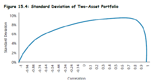
-
Insights from Figure 15.4
- As decreases, portfolio standard deviation decreases.
-
The relationship is nonlinear and asymmetric.
- Negative correlations offer far greater reduction in risk.
- Positive correlations limit diversification.
-
Observation:
- At high positive ρ\rhoρ, optimal portfolio weight may be extreme (e.g., >1 or <0).
- At ρ=−1\rho = -1ρ=−1, it's theoretically possible to completely eliminate risk.
-
Finance Relevance:
- Basis for constructing diversified portfolios.
- Core of Modern Portfolio Theory (MPT) and efficient frontier.
Topic 3. Impact of Correlation on the Standard Deviation
Topic 4. Conditional Expectations
- Definition: The expected value of a random variable , conditioned on a known value of another variable .
X2=x2X_2 = x_2X1X_1
-
Steps to Compute:
- Extract the row from the joint PMF corresponding to .
- Convert that row to a conditional distribution:
- Multiply each possible value of X1X_1 by its conditional probability.
- Sum all products.
-
Interpretation:
-
Helps in scenario analysis: estimating expected return if a certain event occurs.
-
Used in Bayesian modeling, stress testing, and regime switching models.
-
Practice Questions: Q6
Q6. Suppose a portfolio manager creates a conditional PMF based on analyst ratings, X2. Analysts’ ratings can take on three possible outcomes: an upgrade, X2 =1; a downgrade, X2 = –1; or a neutral no change rating, X2 =0. What is the conditional expectation of a return given an analyst upgrade and the following conditional distribution for
A. 2.06%.
B. 3.05%.
C. 4.40%.
D. 11.72%.
Practice Questions: Q6 Answer
Explanation: A is correct.
The conditional expectation of the return given a positive analyst upgrade is computed as:
Module 4. Independent And Identically Distributed Random Variables
Topic 1. Independent and Identically Distributed (i.i.d.) Random Variables
Topic 1. Independent and Identically Distributed (i.i.d.) Random Variables
-
Definition:
- Identically distributed: same mean (μ) and variance (σ²)
- Independent: no mutual influence
- Sum Properties:
- Average:
- Implication: Larger sample size ⇒ Less uncertainty in mean estimate ⇒ Central Limit Theorem begins to apply
Practice Questions: Q7
Q7. Which of the following statements regarding the sums of i.i.d. normal random variables is incorrect?
A. The sums of i.i.d. normal random variables are normally distributed.
B. The expected value of a sum of three i.i.d. random variables is equal to 3μ.
C. The variance of the sum of four i.i.d. random variables is equal to
D. The variance of the sum of i.i.d. random variables grows linearly.
Practice Questions: Q7 Answer
Explanation: C is correct.
The variance of the sum of n i.i.d. random variables is equal to n . Thus, for four i.i.d. random variables, the sum of the variance would be equal to 4 . The covariance terms are all equal to zero because all variables are independent.
Practice Questions: Q8
Q8. The variance of the average of multiple i.i.d. random variables:
A. increases as n increases.
B. decreases as n increases.
C. increases if the covariance is negative as n increases.
D. decreases if the covariance is negative as n increases.
Practice Questions: Q8 Answer
Explanation: B is correct.
The variance of the average of multiple i.i.d. random variables decreases as n increases. The covariance of i.i.d. random variables is always zero.