Book 2. Quantitative Analysis

FRM Part 1

QA 2. Random Variables

Presented by: Sudhanshu

Module 1. Probability Mass Functions, Cumulative Distribution Functions and Expected Values

Module 2. Mean, Variance, Skewness and Kurtosis

Module 3. Probability Density Functions, Quantiles and Linear Transformations

Module 1. Probability Mass Functions, Cumulative Distribution Functions and Expected Values

Topic 1. Random Variables

Topic 2. Probability Mass Function (PMF)

Topic 3. Cumulative Distribution Function (CDF)

Topic 4. Expectations

Topic 1. Random Variables

A random variable assigns a numerical value to each possible outcome of a random process.
Discrete Random Variable: Takes on a countable number of values.
Examples:
- Coin flip: Heads = 1, Tails = 0 (Bernoulli random variable)
- Days in June > 70°F: Values from 0 to 30.
Continuous Random Variable: Takes on an uncountable number of values.
- Example: Amount of rainfall in June — ∞ values possible.
- for any single value; probability measured over intervals, e.g.,

P(X=x)=0

P(6.94 \leq X \leq 6.95)

Topic 2. Probability Mass Function (PMF)

PMF: Gives probability that discrete random variable $X$ takes for a value $x$ .

Bernoulli PMF:
- P(x = 1) = p and P(x = 0) = 1 − p

Uniform Die Roll:

Custom PMF Example:

Validity Condition:

For above example,

f(x)=P(X=x)

f(x)=p^x(1-p)^{1-x}

f(x)=\frac{1}{6}, \quad x=1,2, \ldots, 6

\begin{aligned} & f(x)=\frac{x}{10}, \quad x=1,2,3,4 \\ & P(X=3)=\frac{3}{10}=30 \% \end{aligned}

\sum f\left(x_i\right)=1

\sum f\left(x_i\right)=\frac{1}{10}+\frac{2}{10}+\frac{3}{10}+\frac{4}{10} = \frac{10}{10}=1

Topic 3. Cumulative Distribution Function (CDF)

Definition:
Represents the cumulative probability up to and including $x$ .
For Discrete Variables:

Bernoulli CDF Example (Two outcomes: 0 and 1):
- Let
- Then:

Die Roll Example:
- In general,
F(x) is non-decreasing, piecewise constant for discrete variables.

$\Rightarrow P(X=0) = 1 - p$

P(X=1)=p \Rightarrow P(X=0)=1-p

F(x)=\sum_{x_i \leq x} P\left(X=x_i\right)

F(x)= \begin{cases}0 & \text { if } x<0 \\ 1-p & \text { if } 0 \leq x<1 \\ 1 & \text { if } x \geq 1\end{cases}

F(x)=P(X \leq x)

X=\{1,2,3,4,5,6\}, P(X=x)=\frac{1}{6}

F(3)=P(X \leq 3)=\sum_{x-1}^3 \frac{1}{6}=\frac{3}{6}=0.5

F(x)=\frac{x}{6}, \text { for integer } x \in[1,6]

Practice Questions: Q1

Q1. The probability mass function (PMF) for a discrete random variable that can take on the values 1, 2, 3, 4, or 5 is P(X = x) = x/15. The value of the cumulative distribution function (CDF) of 4, F(4), is equal to:
A. 26.7%.
B. 40.0%.
C. 66.7%.
D. 75.0%.

Practice Questions: Q1 Answer

Explanation: C is correct.

F(4) is the probability that the random variable will take on a value of 4 or less. We can calculate P(X ≤ 4) as 1/15 + 2/15 + 3/15 + 4/15 = 66.7%, or by subtracting 5/15, P(X = 5), from 100% to get 66.7%.

Topic 4. Expectations

Expected Value (Mean):The expected value of a random variable is the probability-weighted average of all possible outcomes.
For a discrete random variable $X$ , with outcomes and corresponding probabilities

Coin Flip: X = 1 for head and 0 for tail,
Die Roll:

Properties of Expectation:
- Scaling:
- Additivity:

$\Rightarrow P(X=0) = 1 - p$

E(X)=(1)(0.5)+(0)(0.5)=0.5

E(X)=\sum_{x-1}^6 x \cdot \frac{1}{6}=\frac{21}{6}=3.5

E(X)=\sum x_i \cdot P\left(x_i\right)

x_1, x_2, \ldots, x_n

p_1, p_2, \ldots, p_n:

E(c X)=c \cdot E(X)

E(X+Y)=E(X)+E(Y)

Practice Questions: Q2

Q2. An analyst has estimated the following probabilities for gross domestic product growth next year:
P(4%) = 10%, P(3%) = 30%, P(2%) = 40%, P(1%) = 20%
Based on these estimates, the expected value of GDP growth next year is:
A. 2.0%.
B. 2.3%.
C. 2.5%.

D. 2.8%.

Practice Questions: Q2 Answer

Explanation: B is correct.

The expected value is computed as: (4)(10%) + (3)(30%) + (2)(40%) + (1)(20%) = 2.3%.

Module 2. Mean, Variance, Skewness and Kurtosis

Topic 1. Central Moments

Topic 2. Variance (2nd moment)

Topic 3. Skewness (3rd moment)

Topic 4. Kurtosis (4th moment)

Topic 1. Central Moments

Moments describe characteristics of the shape of a distribution.
Mean (1st Moment):
General definition:
First Central Moment:
- Always zero, not used in shape analysis.
Why "central"?
- Measured relative to the mean
- Capture shape independent of location
Used to define:
- Variance → 2nd moment,
- Skewness → 3rd moment
- Kurtosis → 4th moment

\mu=E(X)

\mu_k^{\prime}=E\left[(X-\mu)^k\right]

\mu_1^{\prime}=E(X-\mu)=0

Topic 2. Variance

Definition:
Measures:
- Dispersion or spread of a distribution
- Higher variance → outcomes lie farther from mean
Alternative formula:
Standard Deviation (σ):
Preferred due to same units as original data
Example: Suppose

\begin{aligned} E(X)&=1.28 \\ E(X^2)&=(1.8)^2(0.1)+(1.6)^2(0.2)+(1.2)^2(0.4)+(1.0)^2(0.3)=1.6704 \\ Var(X)&=1.6704-(1.28)^2=0.0416 \end{aligned}

\operatorname{Var}(X)=E\left(X^2\right)-[E(X)]^2

\sigma^2=\operatorname{Var}(X)=E\left[(X-\mu)^2\right]

\sigma=\sqrt{E\left[(X-\mu)^2\right]}=\sqrt{\operatorname{Var}(X)}

X=\{1.8,1.6,1.2,1.0\}, \quad P=\{0.1,0.2,0.4,0.3\}

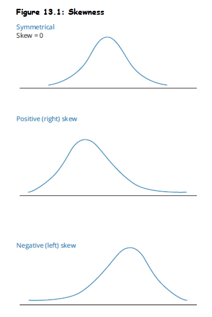
Topic 3. Skewness

Measures: Symmetry of distribution about the mean
Formula:

Interpretation:
- Skew = 0 → Symmetric
- Skew > 0 → Right-skewed (tail on the right)
- Skew < 0 → Left-skewed (tail on the left)
Properties:
- Unitless
- Not affected by linear transformations where $b > 0$
- Reverses sign if scaled by $b < 0$
$$ Example:
- If $μ=2\mu = 2$ , σ = 1, and the third moment is 2:

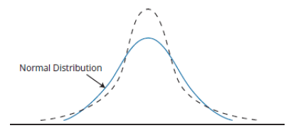
\text { Skewness }=\frac{E\left[(X-\mu)^3\right]}{\sigma^3}

\text { Skewness }=\frac{2}{1^3}=2 \Rightarrow \text { Strong right-skew }

Topic 4. Kurtosis

Definition: Kurtosis measures the "tailedness" of a probability distribution - how much probability is concentrated in the tails versus the center.
Interpretation:
- High Kurtosis → Fat tails → More extreme events
- Low Kurtosis → Light tails → Fewer extreme events
- Mesokurtic: Kurtosis = 3 (normal distribution)
Sometimes Excess Kurtosis is reported:

\text { Excess Kurtosis }=\text { Kurtosis }-3

\text { Kurtosis }=\frac{E\left[(X-\mu)^4\right]}{\sigma^4}

Practice Questions: Q3

Q3. For two financial securities with distributions of returns that differ only in their kurtosis, the one with the higher kurtosis will have:
A. a wider dispersion of returns around the mean.
B. a greater probability of extreme positive and negative returns.
C. less peaked distribution of returns.
D. a more uniform distribution.

Practice Questions: Q3 Answer

Explanation: B is correct.

High kurtosis indicates that the probability in the tails (extreme outcomes) are greater (i.e., the distribution will have fatter tails).

Module 3. Probability Density Functions, Quantiles and Linear Transformations

Topic 1. Probability Density Function (PDF)

Topic 2. Quantile Functions

Topic 3. Linear Transformations of Random Variables

Topic 1. Probability Density Function (PDF)

Defined for Continuous Random Variables
A PDF $f (x)$ gives the relative likelihood that $X$ falls within a small interval around $x.$
For any single point, the probability is zero:
Total Probability:

To Find Probability in an Interval:

The area under the PDF curve over $[a, b]$ gives the probability.
Example: Let $f (x) = 2 x$ for $\in [0,1]$ , 0 otherwise
Then:

P(X=x)=0

\int_{-\infty}^{\infty} f(x) d x=1

P(a \leq X \leq b)=\int_a^b f(x) d x

\int_0^1 2 x d x=\left[x^2\right]_0^1=1

P(0.2 \leq X \leq 0.4)=\int_{0.2}^{0.4} 2 x d x=\left[x^2\right]_{0.2}^{0.4}=0.16-0.04=0.12

Practice Questions: Q4

Q4. Which of the following regarding a probability density function (PDF) is correct? A PDF:
A. provides the probability of each of the possible outcomes of a random variable.
B. can provide the same information as a cumulative distribution function (CDF).
C. describes the probabilities for any random variable.
D. only applies to a discrete probability distribution.

Practice Questions: Q4 Answer

Explanation: B is correct.

A PDF evaluated between minus infinity and a given value gives the probability of an outcome less than the given value; the same information is provided by a CDF. A PDF provides the probabilities only for a continuous random variable. The probability that a continuous random variable will take on a given value is zero.

Topic 2. Quantile Functions

Definition: A quantile function, $Q (p)$ , is the inverse of the cumulative distribution function (CDF).
- Q(p)=x such that F(x)=p
- If $F (2) = 0.30$ , then $Q (0.30)=2$

$\in [0$

Key Quantiles:
Median:
- 50% of outcomes lie below, 50% above
- Equal to the mean in symmetric distributions.
Interquartile Range (IQR):
- Measures spread of central 50% of the distribution.
- Lower IQR = outcomes more concentrated around mean

\mathrm{IQR}=Q(0.75)-Q(0.25)

Q(0.50)=50 \text {th percentile }

Practice Questions: Q5

Q5. For the quantile function, Q(x):
A. the CDF function F[Q(23%)] = 23%.
B. Q(23%) will identify the largest 23% of all possible outcomes.
C. Q(50%) is the interquartile range.
D. x can only take on integer values.

Practice Questions: Q5 Answer

Explanation: A is correct.

Q(23%) gives us a value that is greater than 23% of all outcomes and the CDF for that value is the probability of an outcome less than that value (i.e., 23%).

Topic 3. Linear Transformation of Random Variables

Linear transformation:
Effects:
- Mean:
- Variance:
- Standard Deviation:
- Skewness:
  - $b > 0$ : unchanged
  - $b < 0$ : sign flipped
- Kurtosis: unchanged
- Median and IQR: affected same way as mean and SD
Intuition:
- Shift (a) moves the entire distribution left/right without changing its shape.
- Scale (b) compresses or stretches the distribution and affects spread.
- Negative b reflects the distribution and reverses skew.

Y=a+b X

E(Y)=a+b E(X)

\operatorname{Var}(Y)=b^2 \cdot \operatorname{Var}(X)

\sigma_Y=|b| \cdot \sigma_X

Practice Questions: Q6

Q6. For a random variable, X, the variance of Y = a + bX is:

a^2+b^2 \sigma_x^2

\mathrm{b} \sigma_{\mathrm{x}}^2

\mathrm{b}^2 \sigma_{\mathrm{x}}^2 .

a+b^2 \sigma_x^2

Practice Questions: Q6 Answer

Explanation: C is correct.

The variance of Y is where is the variance of X.

b^2 \sigma_x^2,

\sigma_x^2