Book 2. Quantitative Analysis
FRM Part 1
QA 11. Non-stationary Time Series
Presented by: Sudhanshu
Module 1. Time Trends
Module 2. Seasonality
Module 3. Unit Roots
Module 1. Time Trends

Topic 1. Understanding Time Trends
Topic 2. Linear Trends
Topic 3. Nonlinear Trends
Topic 4. Log-Polynomial and Forecasting
Topic 1. Understanding Time Trends
- Non-stationary time series may exhibit deterministic trends, stochastic trends, or both.
-
Trend Components:
- Deterministic Trend: Includes both time trends and deterministic seasonality.
- Stochastic Trend: Include unit root processes such as random walks.
- Trends can make time series non-stationary, which violates assumptions for standard time series models (like ARMA).
- Objective: Identify and remove trend to obtain a stationary residual series for better modeling.
- Time trends may be linear or nonlinear.
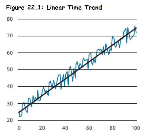
Topic 2. Linear Trends
- A series that exhibits a linear time trend is one that tends to change by the same amount each period.
- Graph shows deviations around a straight line.
- A linear time trend can be modeled as:
-
Limitations
-
Negative value problem: Downward linear trends eventually produce unrealistic negative values when modeling quantities or prices that cannot be negative.
-
Growth rate mismatch: Linear models assume constant absolute increases rather than constant percentage growth, making them unsuitable for variables that naturally grow at steady rates over time.
-
Topic 3. Nonlinear Trends
-
Polynomial Time Trend:
- Models variable growth rates (acceleration or deceleration).
- Flexible, but risk of overfitting.
-
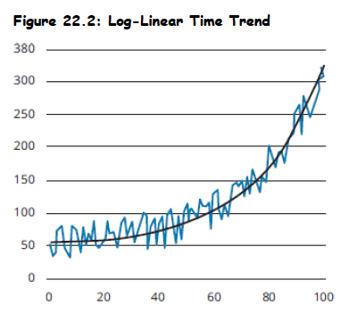
Log-Linear Model:
- Implies a constant percentage growth rate over time.
- Common in economics/finance due to exponential growth in many variables.
Practice Questions: Q1
Q1. An analyst has determined that monthly vehicle sales in the United States have been increasing over the last 10 years, but the growth rate over that period has been relatively constant. Which model is most appropriate to predict future vehicle sales?
A. Linear model.
B. Quadratic model.
C. Log-linear model.
D. Log-quadratic model.
Practice Questions: Q1 Answer
Explanation: C is correct.
A log-linear model is most appropriate for a time series that grows at a relatively constant growth rate.
Topic 4. Log-Polynomial and Forecasting
- Extended Log Models:
- Useful when growth rate itself changes over time.
-
Model Estimation:
- Use Ordinary Least Squares (OLS), assuming εₜ is white noise.
- If εₜ is autocorrelated, OLS results may be biased/inconsistent.
- Forecasting h periods ahead (Linear model):
-
95% Confidence Interval:
- Assumes normal distribution of residuals
-
Detrending:
-
Modeling and removing the trend component results in a detrended time series that we may be able to analyze further.
- Subtract estimated trend from original series.
- Residuals may be modeled with AR, MA, or ARMA if stationary.
-
Practice Questions: Q2
Q2. Using data from 2001 to 2020, an analyst estimates a model for an industry’s annual output as Output = 80.163 + 4.248t + εt, from a regression with a residual standard deviation of 107.574. Assume t equals a given full year (e.g., 2021) and that the error term is normally distributed. A 95% confidence interval for a forecast of 2021
industry output is closest to:
A. 8,374 to 8,796.
B. 8,455 to 8,876.
C. 8,477 to 8,693.
D. 8,557 to 8,773.
Practice Questions: Q2 Answer
Explanation: B is correct.
For t = 2021, a point forecast for industry output is 80.163 + 4.248(2021) = 8,665.371. A 95% confidence interval is 8,665.371 ± 1.96(107.574) = 8,454.526 to 8,876.216.
Module 2. Seasonality
Topic 1. Modeling Seasonality
Topic 2. Forecasting with Seasonality
Topic 1. Modeling Seasonality
- Seasonality: Pattern that repeats periodically (e.g., monthly sales). Can be modeled using seasonal dummy variable regression or seasonal differencing.
-
Calendar Effects: Any cycles that may recur within a year or less.
- Monthly (e.g., December retail surge)
- Quarterly (e.g., earnings season)
- Weekly (e.g., weekend sales effect)
- Seasonal Dummy Variable: Take a value of either 1 or 0 to represent the season being on or off
-
Seasonal Dummy Variable Regression:
- Include k−1 dummies for k seasons (e.g., 3 dummies for 4 quarters).
- The intercept term (β₀) represents the base category (e.g., Q4).
-
Seasonal Differencing:
-
Instead of modeling the level of a series, the differences between its current level and year-ago level are modeled.
-
Seasonal differencing can also help in modeling series with time trends and unit roots.
-
Practice Questions: Q3
Q3. Jill Williams is an analyst in the retail industry. She is modeling a company’s sales and has noticed a quarterly seasonal pattern. If Williams includes an intercept term in her model, how many dummy variables should she use to model the seasonality component?
A. 1.
B. 2.
C. 3.
D. 4.
Practice Questions: Q3 Answer
Explanation: C is correct.
Whenever we want to distinguish between s seasons in a model that incorporates an intercept, we must use s − 1 dummy variables. For example, if we have quarterly data, s = 4, and thus we would include s − 1 = 3 seasonal dummy variables.
Practice Questions: Q4
Q4. Consider the following regression equation utilizing dummy variables for explaining quarterly EPS in terms of the quarter of their occurrence:
The intercept term represents the average value of EPS for the:
A. first quarter.
B. second quarter.
C. third quarter.
D. fourth quarter.
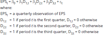
Practice Questions: Q4 Answer
Explanation: D is correct.
The intercept term represents the average value of EPS for the fourth quarter. The slope coefficient on each dummy variable estimates the difference in EPS (on average) between the respective quarter (i.e., quarter one, two, or three) and the omitted quarter (the fourth quarter, in this case).
Topic 2. Forecasting with Seasonality
-
h-step-ahead Point Forecasting:
y^T+h=δ0+δ1(T+h)+βj\hat{y}_{T+h} = \delta_0 + \delta_1(T+h) + \beta_j-
A pure seasonal dummy variable model:
-
After adding a time trend:
-
Adding calendar effects - holiday variations (HDV) and trading-day variations (TDV):
-
-
-
This complete model can now be used for out-of-sample forecasts at time T + h by constructing an h-step-ahead point forecast as follows:
- Set dummy variable to 1 if season i occurs at T+h, else 0.
-
Practice Questions: Q5
Q5. A model for the change in a retailer’s quarterly sales, using seasonal dummy variables DQ, is estimated as:
In the third quarter, sales are forecast to:
A. decrease by 3.8.
B. decrease by 1.0.
C. increase by 1.1.
D. increase by 3.8.
Practice Questions: Q5 Answer
Explanation: C is correct.
Module 3. Unit Roots
Topic 1. Random Walk and Unit Root
Topic 2. Challenges & Testing for Unit Roots
Topic 1. Random Walk and Unit Root
-
Random Walk:
-
Every observation = prior value plus-or-minus shock.
-
Not mean-reverting, variance increases over time.
-
No long-term equilibrium.
-
It is not covariance stationary, so cannot be modeled using AR, MA or ARMA processes.
-
-
Back-substitution:
-
Entire history of shocks affects current value.
-
Unit Root:
-
When expressing using lag polynomials, one of their roots is 1.
-
Example:
-
A random walk is a special case of unit roots.
-
A unit root process is sometimes described as a random walk with drift.
-
We can think of random walk and unit root interchangeably in this chapter.
-
Practice Questions: Q6
Q6. A random walk is most accurately described as a time series whose value is a function of its:
A. previous value only.
B. beginning value only.
C. previous value and a random shock.
D. beginning value and all historical shocks.
Practice Questions: Q6 Answer
Explanation: D is correct.
For a random walk, so its value at time t is a function of its beginning value and all shocks, as well as the shock in the observation’s own period.
Topic 2. Challenges & Testing for Unit Roots
-
Challenges:
-
Unlike stationary time series, a series with a unit root does not revert to a mean.
-
Time series with unit roots often show spurious relationships with each other.
-
If we use an ARMA model, its estimated parameters follow an asymmetric distribution that depends on the sample size and the presence of a time trend (a Dickey-Fuller distribution). This reduces our ability to select a correct model or make valid forecasts.
-
-
Remedy:
-
Use 1st differencing:
-
If still non-stationary, use 2nd differencing.
-
-
Augmented Dickey-Fuller (ADF) Test:
-
-
-
γ represents the coefficient on lagged value.
-
Reject H₀ if γ is significantly negative.
-
Practice Questions: Q7
Q7. An augmented Dickey-Fuller test will reject the hypothesis that a process is a unit root if the coefficient on the lagged value is statistically significantly:
A. less than zero.
B. equal to zero.
C. greater than zero.
D. different from zero.
Practice Questions: Q7 Answer
Explanation: A is correct.
Although the null hypothesis is that the coefficient on the lagged value is equal to zero, the rejection condition is that the coefficient is less than zero.