Book 2. Quantitative Analysis
FRM Part 1
QA 10. Stationary Time Series
Presented by: Sudhanshu
Module 1. Covariance Stationary
Module 2. Autoregressive (AR) and Moving Average (MA) Models
Module 3. Autoregressive Moving Average (ARMA) Models
Module 1. Covariance Stationary

Topic 1. Covariance Stationarity Conditions
Topic 2. Autocovariance and Autocorrelation Functions
Topic 3. White Noise
Topic 1. Covariance Stationarity Conditions
- Time Series Definition: Data collected over regular time periods (e.g., monthly S&P 500 returns, quarterly dividends paid by a company)
- Time Series Components:
- Trend: component that changes over time
- Seasonality: systematic changes occurring at specific times of the year
- Cyclicality: changes occurring over time cycles (focus of this analysis)
- Cyclical Component Decomposition: Can be broken into shocks and persistence components; linear models are used to model the persistence component
- Covariance Stationarity: A time series property where relationships among present and past values remain stable over time, enabling forecasting based on historical values
- Three Properties of Covariance Stationarity:
- Mean must be stable over time
- Variance must be finite and stable over time
- Covariance structure must be stable over time
- Covariance Structure: Refers to covariances among time series values at various lags (given number of periods apart)
- Lag Notation: Represented by lowercase Greek letter tau (τ):
- τ = 1: one-period lag comparing each value to its preceding value
- τ = 4: comparing values four periods apart along the time series
Practice Questions: Q1
Q1. The conditions for a time series to exhibit covariance stationarity are least likely to include:
A. a stable mean.
B. a finite variance.
C. a finite number of observations.
D. autocovariances that do not depend on time.
Practice Questions: Q1 Answer
Explanation: C is correct.
In theory, a time series can be infinite in length and still be covariance stationary. To be covariance stationary, a time series must have a stable mean, a stable covariance structure (i.e., autocovariances depend only on displacement, not on time), and an infinite variance.
Topic 2. Autocovariance and Autocorrelation Functions
- Autocovariance at Lag τ: The covariance between the current value of a time series and its value τ periods in the past
- Autocovariance Function: The complete set of autocovariances for all lag values (τ); stable over time for covariance stationary series, depending only on lag τ, not on the observation period
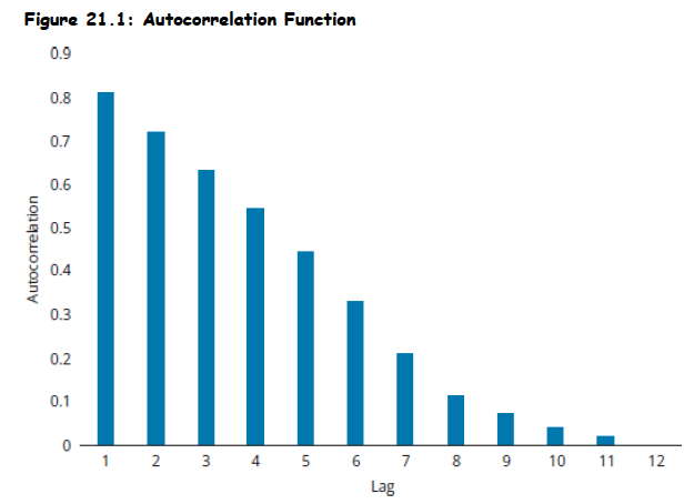
- Autocorrelation Function (ACF): Created by dividing each autocovariance by the variance of the time series, producing autocorrelations scaled between -1 and +1 for better interpretation of relationship strength
- ACF Graphical Analysis: Fig 21.1 shows an ACF where autocorrelations approach zero as lag τ increases, a characteristic always present in covariance stationary series
Topic 2. Autocovariance and Autocorrelation Functions
- Partial Autocorrelation Function: Correlations for all lags after controlling for values between the lags (similar to regression coefficients when including all lags as independent variables)
- ACF vs. Partial Autocorrelation Patterns:
- Autocorrelations decline successively and gradually
- Partial autocorrelations experience steep decline and may be large only for a few specific lags
- Large partial autocorrelations at certain lags become prime candidates for inclusion in autoregressive (AR) models
Practice Questions: Q2
Q2. As the number of lags or displacements becomes large, autocorrelation functions (ACFs) will approach:
A. −1.
B. 0.
C. 0.5.
D. +1.
Practice Questions: Q2 Answer
Explanation: B is correct.
One feature that all ACFs have in common is that autocorrelations approach zero as the number of lags or displacements gets large.
Topic 3. White Noise
- Serially Uncorrelated Time Series: A time series exhibiting zero correlation among any of its lagged values
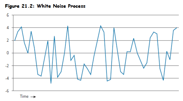
- White Noise Process: A serially uncorrelated series with mean of zero and constant variance (also called zero-mean white noise)
- Independent White Noise: A white noise process where observations are both independent and uncorrelated
- Normal/Gaussian White Noise: Independent white noise that follows a normal distribution; all normal white noise processes are independent white noise, but not all independent white noise processes are normally distributed
- Graphical Representation: A white noise process resembles Figure 21.2, showing no identifiable patterns among time periods
Topic 3. White Noise
- Forecasting Model Analysis: A model's forecast errors should follow a white noise process; if errors can be forecasted based on past values, the model is inaccurate in a predictable way and requires revision (e.g., adding more lags)
- Unconditional vs. Conditional Moments:
- White noise has constant unconditional mean (zero) and variance
- Conditional mean and variance may vary based on earlier values, enabling forecasting
- Independent white noise has conditional mean equal to unconditional mean, making forecasting from past values impossible
- Wold's Theorem and General Linear Process: A covariance stationary process can be modeled as an infinite distributed lag of a white noise process:
- Formula:
-
where b variables are constant and is a white noise process
-
As this expression can be applied to any covariance stationary series, it is known as a general linear process.
- Formula:
Practice Questions: Q3
Q3. Which of the following statements about white noise is most accurate?
A. All serially uncorrelated processes are white noise.
B. All Gaussian white noise processes are independent white noise.
C. All independent white noise processes are Gaussian white noise.
D. All serially correlated Gaussian processes are independent white noise.
Practice Questions: Q3 Answer
Explanation: B is correct.
If a white noise process is Gaussian (i.e., normally distributed), it follows that the process is independent white noise. However, the reverse is not true; there can be independent white noise processes that are not normally distributed. Only those serially uncorrelated processes that have a zero mean and constant variance are white noise.
Module 2. Autoregressive And Moving Average Models
Topic 1. Autoregressive Processes
Topic 2. Estimating Autoregressive Parameters using Yule-Walker Equation
Topic 3. Moving Average (MA) Processes
Topic 4. Lag Operators
Topic 1. Autoregressive Processes
- Most widely applied time series models in finance.
- First-Order Autoregressive [AR(1)] Process: A variable regressed against itself in lagged form:
- d: intercept term
- yt: time series variable being estimated
- : one-period lagged observation of the variable being estimated
- : current random white noise shock (mean 0)
- Φ: coefficient for the lagged observation of the variable being estimated
- Covariance Stationarity for AR(1): Absolute value of the coefficient on the lagged operator must be < 1 (∣Φ∣<1).
- Covariance Stationarity for AR(p): The sum of all coefficients should be < 1.
- Long-Run (Unconditional) Mean Reverting Level:
- For an AR(1) series:
- For an AR(p) series:
- For an AR(1) series:
- This mean reverting level acts as an attractor, drawing the time series toward its mean over time.
- VarianVaVariance for AR(1): Variance of
Practice Questions: Q4
Q4. Which of the following conditions is necessary for an autoregressive (AR) process to be covariance stationary?
A. The value of the lag slope coefficients should add to 1.
B. The value of the lag slope coefficients should all be less than 1.
C. The absolute value of the lag slope coefficients should be less than 1.
D. The sum of the lag slope coefficients should be less than 1.
Practice Questions: Q4 Answer
Explanation: D is correct.
In order for an AR process to be covariance stationary, the sum of each of the slope coeficients should be less than 1.
Topic 2. Estimating Autoregressive Parameters using Yule-Walker Equation
- Forecasters estimate autoregressive parameters by accurately estimating the autocovariance function of the data series:
- Yule-Walker Equation: Used to estimate the autoregressive parameters
- For AR(1) process, the foolowing relationship is used:
- for t=0,1,2,...
- Significance: For autoregressive processes, autocorrelation decays geometrically to zero as t increases.
- Example: For , the first-period autocorrelation is , and the second-period autocorrelation is , and so on.
- If Φ is negative, the autocorrelation will still decay in absolute value but oscillate between negative and positive numbers.
Topic 3. Moving Average (MA) Processes
- Definition: A linear regression of the current values of a time series against both the current and previous unobserved white noise error terms (random shocks).
- Covariance Stationarity: MA processes are always covariance stationary.
- First-Order Moving Average [MA(1)] Process: Only 1 lagged-error term.
-
- μ: mean of the time series
- : current random white noise shock (mean 0)
- : one-period lagged random white noise shock
- θ : coefficient for the lagged random shock
-
- Short-Term Memory: An MA(1) process has short-term memory because it only incorporates what happened one period ago.
- Autocorrelation Cutoff: The autocorrelation is computed using the formula:
-
For any value beyond the first lagged error term, the autocorrelation will be zero in an MA(1) process. It is one condition of being covariance stationary.
-
A more general form, MA(q), incorporates q lags:
-
Mean of MA(q) is still μ but the variance,
Practice Questions: Q5
Q5. Which of the following statements is a key differentiator between a moving average (MA) representation and an autoregressive (AR) process?
A. An MA representation shows evidence of autocorrelation cutoff.
B. An AR process shows evidence of autocorrelation cutoff.
C. An unadjusted MA process shows evidence of gradual autocorrelation decay.
D. An AR process is never covariance stationary.
Practice Questions: Q5 Answer
Explanation: A is correct.
A key difference between an MA representation and an AR process is that the MA process shows autocorrelation cutoff while an AR process shows a gradual decay in autocorrelations.
Practice Questions: Q6
Q6. Assume in an autoregressive [AR(1)] process that the coefficient for the lagged observation of the variable being estimated is equal to 0.75. According to the Yule-Walker equation, what is the second-period autocorrelation?
A. 0.375.
B. 0.5625.
C. 0.75.
D. 0.866.
Practice Questions: Q6 Answer
Explanation: B is correct.
The coefficient is equal to 0.75, so using the concept derived from the Yule-Walker equation, the first-period autocorrelation is 0.75 (i.e., ), and the second- period autocorrelation is 0.5625.
Topic 4. Lag Operators
- Notation: A commonly used notation in time series modeling (L).
- Function: Shifts the time index back by one period:
- Six Properties of Lag Operator:
- Shifts the time index back by one period.
- (multiple periods).
- Does not change a constant when applied.
- Used in lag polynomials to assign weights to past values
- Example: If we have the model
- Using lag operators in this model (known as a lag polynomial), it would be expressed as:
- Lag polynomials can be multiplied.
- Can be inverted if coefficients satisfy certain conditions.
- Main Purposes:
- An AR process is covariance stationary only if its lag polynomial is invertible.
- Invertibility is used in the Box-Jenkins methodology to select the appropriate time series model.
Practice Questions: Q7
Q7. Which of the following statements is most likely a purpose of the lag operator?
A. A lag operator ensures that the parameter estimates are consistent.
B. An autoregressive (AR) process is covariance stationary only if its lag polynomial is invertible.
C. Lag polynomials can be multiplied.
D. A lag operator ensures that the parameter estimates are unbiased.
Practice Questions: Q7 Answer
Explanation: B is correct.
There are two main purposes of using a lag operator. First, an AR process is covariance stationary only if its lag polynomial is invertible. Second, this invertibility is used in the Box-Jenkins methodology to select the appropriate time series model.
Module 3. Autoregressive Moving Average (ARMA) Models
Topic 1. Autoregressive Moving Average (ARMA) Processes
Topic 2. Application of AR, MA, and ARMA Processes
Topic 3. Sample and Partial Autocorrelations
Topic 4. Testing Autocorrelations
Topic 5. Modeling Seasonality in an ARMA
Topic 1. Autoregressive Moving Average (ARMA) Processes
- Autoregressive Moving Average Processes: Combines both autoregressive (AR) and moving average (MA) processes to capture richer relationships in a time series.
- Formula (ARMA(1,1)):
-
- d: intercept term
- yt: time series variable
- Φ: coefficient for lagged observations (yt−1)
- : current random white noise shock
- θ: coefficient for lagged random shocks ( )
-
- Covariance Stationarity: For an ARMA process to be covariance stationary, ∣Φ∣<1.
- Autocorrelation Decay: Autocorrelations in an ARMA process will also decay gradually.
- ARMA(p,q) Model: Represents 'p' lagged operators in the AR portion and 'q' lagged operators in the MA portion.
- Offers the highest possible set of combinations for time series forecasting.
Practice Questions: Q8
Q8. Which of the following statements about an autoregressive moving average (ARMA) process is correct?
I. It involves autocorrelations that decay gradually.
II. It combines the lagged unobservable random shock of the MA process with the observed lagged time series of the AR process.
A. I only.
B. II only.
C. Both I and II.
D. Neither I nor II.
Practice Questions: Q8 Answer
Explanation: C is correct.
The ARMA process is important because its autocorrelations decay gradually and because it captures a more robust picture of a variable being estimated by including both lagged random shocks and lagged observations of the variable being estimated. The ARMA model merges the lagged random shocks from the MA process and the lagged time series variables from the AR process.
Topic 2. Application of AR, MA, and ARMA Processes
- Model Selection Using Autocorrelations:
- Abrupt cutoff in autocorrelations suggests using an MA process
- Gradual decay in autocorrelations suggests using AR or ARMA process
- Periodic spikes during gradual decay (e.g., every 12th autocorrelation jumps upward) indicate seasonality effects, pointing toward AR or ARMA models
- Practical Model Testing: Test various models using regression results, particularly for data with seasonality patterns such as employment data; moving average processes are typically not robust for real-world data with gradually decaying autocorrelations
- AR(2) Model Structure: Base model includes constant value (μ) when all other values are zero
- Generic Formula:
-
- Applied Example:
-
- Generic Formula:
Topic 2. Application of AR, MA, and ARMA Processes
- ARMA(3,1) Model Structure: Combines autoregressive and moving average components for seasonally impacted data Generic Formula:
- Generic Formula:
-
- Applied Example:
-
- Forecasting Example Using ARMA(3,1): Given previous values , and previous shock :
-
-
-
- Generic Formula:
- Model Comparison: Researchers determine whether AR(2) or ARMA(3,1) provides better predictions for seasonally impacted data series
Practice Questions: Q9
Q9. Which of the following statements is correct regarding the usefulness of an
autoregressive (AR) process and an autoregressive moving average (ARMA) process when modeling seasonal data?
I. They both include lagged terms and, therefore, can better capture a relationship
in motion.
II. They both specialize in capturing only the random movements in time series data.
A. I only.
B. II only.
C. Both I and II.
D. Neither I nor II
Practice Questions: Q9 Answer
Explanation: A is correct.
Both AR models and ARMA models are good at forecasting with seasonal patterns because they both involve lagged observable variables, which are best for capturing a relationship in motion. It is the moving average representation that is best at capturing only random movements.
Topic 3. Sample and Partial Autocorrelations
- Sample Autocorrelation and Partial Autocorrelation: Calculated using sample data.
- Purpose: Used to validate and improve ARMA models.
- Model Selection: Initially, these statistics guide the analyst in selecting an appropriate model.
- Goodness of Fit Evaluation: Residual autocorrelations at different lags are computed and tested for statistical significance.
- If the model fits well, none of the residual autocorrelations should be statistically significantly different from zero, indicating whether the model has captured all information or whether some information is still present in the residuals.
Topic 4. Testing Autocorrelations
- Model Specification Checks: Involve examining residual Autocorrelation Function (ACF).
- Goal: All residual autocorrelations should be zero.
- Graphical Examination: Autocorrelations violating the 95% confidence interval around zero indicate the model does not adequately capture underlying patterns.
- Joint Tests for Residual Autocorrelations:
- Box-Pierce (BP) Q statistic: A joint test to determine if all residual autocorrelations equal zero versus at least one is not equal to zero.
-
- Ljung-Box (LB) Q statistic: A version of the BP statistic that works better for smaller samples (T ≤ 100).
- Where:
- Q is a chi-squared statistic with h degrees of freedom
- T is the sample size
- is the sample autocorrelation at lag i
- Box-Pierce (BP) Q statistic: A joint test to determine if all residual autocorrelations equal zero versus at least one is not equal to zero.
Practice Questions: Q10
Q10. To test the hypothesis that the autocorrelations of a time series are jointly equal to zero based on a small sample, an analyst should most appropriately calculate:
A. a Ljung-Box (LB) Q-statistic.
B. a Box-Pierce (BP) Q-statistic.
C. either a Ljung-Box (LB) or a Box-Pierce (BP) Q-statistic.
D. neither a Ljung-Box (LB) nor a Box-Pierce (BP) Q-statistic.
Practice Questions: Q10 Answer
Explanation: A is correct.
The LB Q-statistic is appropriate for testing this hypothesis based on a small sample.
Topic 5. Modeling Seasonality in an ARMA
- Seasonality: Recurrence of a pattern at the same time every year (e.g., higher retail sales in Q4).
- Modeling in Pure AR Process: Include a lag corresponding to the seasonality (e.g., 4th lag for quarterly data, 12th for monthly data) in addition to other short-term lags.
- Modeling in Pure MA Process: A similar approach is used.
- ARMA Model with Seasonality Notation: ARMA
- and denote the seasonal component.
- and are restricted to values of 1 or 0 (true or false), where 1 corresponds to the seasonal lag (e.g., 12 for monthly).