Book 1. Market Risk
FRM Part 2
MR 1. Estimating Market Risk Measures
Presented by: Sudhanshu
Module 1. Historical and Parametric Estimation Approaches
Module 2. Risk Measures
Module 1. Historical and Parametric Estimation Approaches
Topic 1. Estimating Returns: Key Concepts
Topic 2. Historical Simulation Approach to VaR (HSVaR)
Topic 3. HSVaR: Examples Of VaR Limit and VaR Estimation
Topic 4. Parametric Estimation Approaches
Topic 5. Parametric VaR: Normal VaR Overview
Topic 6. Parametric VaR: Normal VaR Examples
Topic 7. Parametric VaR: Lognormal VaR Overview
Topic 8. Parametric VaR: Lognormal VaR Examples

Topic 1. Estimating Returns: Key Concepts
-
The convention in risk management is to quote return losses as positive values for clarity. For example, a loss of $1 million would be stated as "a loss of $1 million," not "a profit of −$1 million."
-
Profit/Loss Data ( ): This is the most direct way to measure a change in value. It represents the change in the value of an asset or portfolio from one period to the next, including any interim payments like dividends or interest.
-
-
-
Arithmetic Returns ( ): Also known as simple returns, this method is useful for single-period analysis. It assumes that any interim payments are not reinvested. Because of this, it is not suitable for longer investment horizons where the compounding effect of reinvestment becomes important.
-
-
Geometric Returns ( ): Also known as continuously compounded returns, this method is more appropriate for multi-period analysis. It assumes that all interim payments are continuously reinvested. This approach is preferred for its mathematical tractability and because it ensures that the asset price can never become negative.
Topic 2. Historical Simulation Approach to VaR (HSVaR)
-
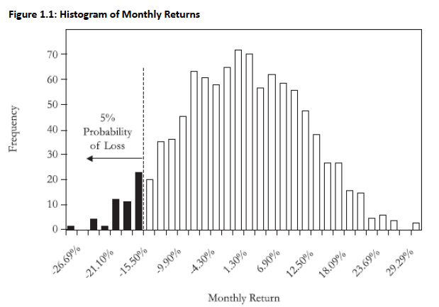
Calculation Process
- Order return observations from largest to smallest
- Find observation separating tail from body of distribution
- VaR observation at (1 − α) confidence level = (α × n) + 1
-
Example (n=1, 95% confidence): Lower tail = lowest 5% of returns; 95% VaR = -15.5% return
- For $1M investment: one-month VaR = $155,000
-
Limitations
- Assumes future returns follow same generating process as past
- Cannot adjust for changing economic conditions
- Unable to accommodate abrupt parameter shifts
Topic 3. HSVaR: Examples Of VaR Limit and VaR Estimation
-
Example (Identifying the VaR limit): Identify the ordered observation in a sample of 1,000 data points that corresponds to VaR at a 95% confidence level.
-
Solution: Since VaR is to be estimated at 95% confidence, this means that 5% (i.e., 50) of the ordered observations would fall in the tail of the distribution. Therefore, the 51st ordered loss observation would separate the 5% of largest losses from the remaining 95% of returns.
-
Example (Computing VaR): A long history of profit/loss data closely approximates a standard normal distribution (mean equals zero; standard deviation equals one). Estimate the 5% VaR using the historical simulation approach.
-
Solution: The VaR limit will be at the observation that separates the tail loss with area equal to 5% from the remainder of the distribution. Since the distribution is closely approximated by the standard normal distribution, the VaR is 1.65 (5% critical value from the z-table). Recall that since VaR is a one tailed test, the entire significance level of 5% is in the left tail of the returns distribution.
Practice Questions: Q1
Q1. The VaR at a 95% confidence level is estimated to be 1.56 from a historical simulation of 1,000 observations. Which of the following statements is most likely true?
A. The parametric assumption of normal returns is correct.
B. The parametric assumption of lognormal returns is correct.
C. The historical distribution has fatter tails than a normal distribution.
D. The historical distribution has thinner tails than a normal distribution.
Practice Questions: Q1 Answer
Explanation: D is correct.
The historical simulation indicates that the 5% tail loss begins at 1.56, which is less than the 1.65 predicted by a standard normal distribution. Therefore, the historical simulation has thinner tails than a standard normal distribution.
Practice Questions: Q2
Q2. Assume the profit/loss distribution for XYZ is normally distributed with an annual mean of $20 million and a standard deviation of $10 million. The 5% VaR is calculated and interpreted as which of the following statements?
A. 5% probability of losses of at least $3.50 million.
B. 5% probability of earnings of at least $3.50 million.
C. 95% probability of losses of at least $3.50 million.
D. 95% probability of earnings of at least $3.50 million.
Practice Questions: Q2 Answer
Explanation: D is correct.
The value at risk calculation at 95% confidence is: −20 million + 1.65 × 10 million = −$3.50 million. Since the expected loss is negative and VaR is an implied negative amount, the interpretation is that XYZ will earn less than +$3.50 million with 5% probability, which is equivalent to XYZ earning at least $3.50 million with 95% probability.
Topic 4. Parametric Estimation Approaches
-
The parametric approach (e.g., the delta-normal approach) explicitly assumes a distribution for the underlying observations.
-
We will analyze two cases:
-
VaR for returns that follow a normal distribution, and
-
VaR for returns that follow a lognormal distribution
-
Topic 5. Parametric VaR: Normal VaR Overview
-
Conceptual Understanding
- VaR separates tail losses from remaining distribution at given confidence level
- VaR cutoff located in left tail of returns distribution
- Calculated value is negative but reported as positive (negative amount implied)
-
Formula
-
For P/L data:
-
where μ and σ denote the mean and standard deviation of the profit/loss distribution and z denotes the critical value (i.e., quantile) of the standard normal distribution.
-
-
In practice, the population parameters μ and σ are not likely known, in which case the researcher will use the sample mean and standard deviation.
- For arithmetic return data:
-
For P/L data:
Topic 6. Parametric VaR: Normal VaR Examples
-
Example (Computing VaR (P/L distribution)): Assume that the profit/loss distribution for XYZ is normally distributed with an annual mean of $15 million and a standard deviation of $10 million. Calculate the VaR at the 95% and 99% confidence levels using a parametric approach.
-
Solution:
-
VaR(5%) = −$15 million + $10 million × 1.65 = $1.5 million. Therefore, XYZ expects to lose at most $1.5 million over the next year with 95% confidence. Equivalently, XYZ expects to lose more than $1.5 million with a 5% probability.
-
VaR(1%) = −$15 million + $10 million × 2.33 = $8.3 million. Note that the VaR (at 99% confidence) is greater than the VaR (at 95% confidence) as follows from the definition of value at risk.
-
-
Example (Computing VaR (arithmetic returns)): A portfolio has a beginning period value of $100. The arithmetic returns follow a normal distribution with a mean of 10% and a standard deviation of 20%. Calculate VaR at both the 95% and 99% confidence levels.
-
Solution:
-
VaR(5%) = (−10% + 1.65 × 20%) × 100 = $23.0.
-
VaR(1%) = (−10% + 2.33 × 20%) × 100 = $36.6.
-
Topic 7. Parametric VaR: Lognormal VaR Overview
-
Lognormal Distribution Properties
- Right-skewed with positive outliers
- Bounded below by zero (prevents negative asset prices)
-
Relationship to Returns and Prices: If geometric returns follow normal distribution , then follows normal distribution and follows lognormal distribution:
-
-
Application
- Commonly used to prevent modeling negative asset prices
- VaR can be derived through algebraic manipulation of these relationships
-
Note: The calculation of lognormal VaR (geometric returns) and normal VaR
(arithmetic returns) will be similar when we are dealing with short time periods and practical return estimates.
Topic 8. Parametric VaR: Lognormal VaR Examples
-
Example (Computing VaR (Lognormal distribution)): A diversified portfolio exhibits a normally distributed geometric return with mean and standard deviation of 10% and 20%, respectively. Calculate the 5% and 1% lognormal VaR assuming the beginning period portfolio value is $100.
-
Solution:
Module 2. Risk Measures
Topic 1. Expected Shortfall (ES): Overview
Topic 2. Expected Shortfall (ES): Example
Topic 3. Coherent Risk Measures: Overview
Topic 4. Coherent Risk Measures: Convergence and Standard Errors
Topic 5. Estimating Standard Errors: Example
Topic 6. Coherent Risk Measures: Variance Approximation
Topic 7. Quantile-Quantile (QQ) Plots
-
Limitation of VaR:
-
VaR gives only the maximum loss at a given confidence level.
-
It does not show the magnitude of losses beyond that threshold.
-
-
Expected Shortfall (ES):
-
Also called Conditional VaR (CVaR).
-
Estimates average loss in the tail beyond the VaR level.
-
Computed by dividing the tail distribution into n equal slices and averaging the corresponding VaRs.
-
Topic 1. Expected Shortfall (ES): Overview
Topic 2. Expected Shortfall (ES): Example
-
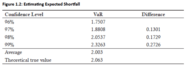
Example (n = 5, Normal distribution):
-
Tail split into 5 slices.
-
Compute 4 VaRs (for increasing confidence levels).
-
ES = average of these tail VaRs → gives a better picture of extreme losses.
-
- VaR increases (from the Difference column) to maintain the same 1% interval mass because the tails get thinner with higher nnn.
-
Avg of 4 VaRs = 2.003, which represents the ES (probability-weighted tail loss)
-
As nnn increases, the ES rises and converges to the true theoretical loss (2.063).
-
With large nnn (e.g., >10,000), the avg of many VaRs approaches the theoretical ES.
Topic 3. Coherent Risk Measures: Overview
-
Definition: Weighted average of loss distribution quantiles based on user-specific risk aversion
-
More general than VaR or ES; ES is a special case
-
ES uses constant weighting [1/(1 − confidence level)] for tail losses only; other quantiles weighted at zero
-
- Methodology: Entire distribution divided into equal probability slices (not just tail region like ES). Each slice weighted by risk aversion function and averaged
-
Coherent Risk Measure Calculation (n=10 Example):
-
Step 1: Divide Distribution:
- Split return distribution into 9 equal probability slices (n − 1)
- Breakpoints at 10%, 20%, ..., 90% quantiles
-
Step 2: Identify Quantile Values:
- 10% quantile → -1.2816,
- 20% quantile → -0.8416,
- 90% quantile → 1.2816
-
Step 3: Calculate Risk Measure:
- Weight each quantile by risk aversion function
- Average weighted quantiles to obtain coherent risk measure value
-
Step 1: Divide Distribution:
-
Convergence Properties:
- More sensitive to choice of n than ES
- Converges to true value with sufficiently large n
- Higher n pushes quantiles into distribution tails where extreme values exist
-
Find optimal n:
- Start with small n, double repeatedly until estimates stabilize
- Doubling n halves the width of tail slices
- Calculate "halving error" (difference between consecutive estimates)
- Optimal n achieved when halving error ≈ 0
-
Estimating Standard Errors: It is important to compute the standard error for risk measure estimators to understand their precision. The formula for the standard error of a quantile is:
-
-
-
Here, p is the left-tail probability, n is the sample size and f(q) is the probability mass.
-
-
A confidence interval based on standard error is given by:
- Here, q is the quantile value, is the critical value and se(q) is the standard error.
Topic 4. Coherent Risk Measures: Convergence and Standard Errors
- Example: Construct a 90% confidence interval for 5% VaR (the 95% quantile) drawn from a standard normal distribution. Assume bin width = 0.1 and that the sample size is equal to 500.
-
Solution:
- The quantile value, q, corresponds to the 5% VaR which occurs at 1.65 for the standard normal distribution. The confidence interval takes the following form: [1.65 + 1.65*se(q)]>VaR>[1.65 - 1.65*se(q)]
-
Since bin width is 0.1, q is in the range 1.65 ± 0.1/2 = [1.7, 1.6]. Note that the left tail probability, p, is the area to the left of −1.7 for a standard normal distribution.
-
Next, calculate the probability mass between [1.7, 1.6], represented as f(q). From the standard normal table, the probability of a loss greater than 1.7 is 0.045 (left tail). Similarly, the probability of a loss less than 1.6 (right tail) is 0.945. Collectively, f(q) = 1 − 0.045 − 0.945 = 0.01.
-
The standard error of the quantile is derived from the variance approximation of q and is equal to:
-
- Thus, the confidence interval for VaR is given by:
Topic 5. Estimating Standard Errors: Example
Topic 6. Coherent Risk Measures: Variance Approximation
-
Increasing Sample Size (n)
- Standard error decreases
- Confidence interval narrows
-
Increasing Bin Size
- Probability mass f(q) increases
- Left tail probability (p) decreases
- Standard error decreases
- Confidence interval narrows
-
Increasing Tail Probability (p)
- Estimator becomes less precise
- Standard errors increase
- Confidence interval widens
- Note: p(1 − p) maximized at p = 0.5
Practice Questions: Q1
Q1. Which of the following statements about expected shortfall estimates and coherent risk measures are true?
A. Expected shortfall and coherent risk measures estimate quantiles for the entire loss distribution.
B. Expected shortfall and coherent risk measures estimate quantiles for the entire loss distribution.
C. Expected shortfall estimates quantiles for the tail region and coherent risk measures estimate quantiles for the non-tail region only.
D. Expected shortfall estimates quantiles for the entire distribution and coherent risk measures estimate quantiles for the tail region only.
Practice Questions: Q1 Answer
Explanation: B is correct.
ES estimates quantiles for n − 1 equal probability masses in the tail region only. The coherent risk measure estimates quantiles for the entire loss distribution.
Practice Questions: Q2
Q2. Which of the following statements most likely increases standard errors from coherent risk measures?
A. Increasing sample size and increasing the left tail probability.
B. Increasing sample size and decreasing the left tail probability.
C. Decreasing sample size and increasing the left tail probability.
D. Decreasing sample size and decreasing the left tail probability.
Practice Questions: Q2 Answer
Explanation: C is correct.
Decreasing sample size clearly increases the standard error of the coherent risk measure given that standard error is defined as:
As the left tail probability, p, increases, the probability of tail events increases, which also increases the standard error. Mathematically, p(1 − p) increases as p increases until p = 0.5. Small values of p imply smaller standard errors.
Topic 7. Quantile-Quantile (QQ) Plots
-
Purpose & Methodology
- Visual tool to examine if empirical data fits theoretical distribution (e.g., standard normal)
- Plots empirical quantiles against theoretical quantiles at regular confidence intervals
-
Interpretation: Similar Distributions
- If data from same distribution, empirical median plots near zero (theoretical median = exactly zero)
- Plotting multiple quantiles (40%, 60%, etc.) creates linear QQ plot when distributions closely match
-
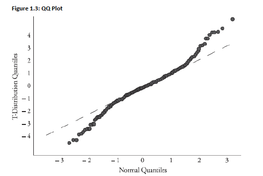
Example: t-Distribution vs. Normal
- Both symmetric, but t-distribution has fatter tails
- Near median (50% confidence): quantiles align closely
-
In tails: quantiles diverge
- 95% confidence: z = -1.65 vs. t ≈ -1.68 (df ≈ 40)
- 97.5% confidence: z = -1.96 vs. t = -2.02
-
General Interpretation Rule: Middle matches, tails diverge → empirical distribution is symmetric with non-normal tails (fatter or thinner)
- The QQ plot is given below:
Topic 8. Quantile-Quantile (QQ) Plots
Practice Questions: Q3
Q3. The quantile-quantile plot is best used for what purpose?
A. Testing an empirical distribution from a theoretical distribution.
B. Testing a theoretical distribution from an empirical distribution.
C. Identifying an empirical distribution from a theoretical distribution.
D. Identifying a theoretical distribution from an empirical distribution.
Practice Questions: Q3 Answer
Explanation: C is correct.
Once a sample is obtained, it can be compared to a reference distribution for possible identification. The QQ plot maps the quantiles one to one. If the relationship is close to linear, then a match for the empirical distribution is found. The QQ plot is used for visual inspection only without any formal statistical test.