Book 1. Market Risk
FRM Part 2
MR 2. Non-Parametric Approaches
Presented by: Sudhanshu
Module 1. Nonparametric Approaches
Module 1. Nonparametric Approaches
Topic 1. Nonparametric Approaches
Topic 2. Bootstrap Historical Simulation Approach
Topic 3. Applying Nonparametric Estimation
Topic 4. Weighted Historical Simulation Approaches
Topic 5. Age-Weighted Historical Simulation
Topic 6. Volatility-Weighted Historical Simulation
Topic 7. Correlation-Weighted Historical Simulation
Topic 8. Filtered Historical Simulation
Topic 9. Advantages of Nonparametric Methods
Topic 10. Disadvantages of Nonparametric Methods

Topic 1. Nonparametric Approaches
-
Non-parametric estimation is not assumption-driven; it does not make restrictive assumptions (like Normal or Log-Normal) about the underlying data distribution.
-
Flexibility: Allows the data to drive the estimation, making it suitable for VaR (Value at Risk) estimation, especially when tail events are sparse.
Topic 2. Bootstrap Historical Simulation Approach
-
Bootstrap Methodology
- Draw sample from original data set
- Calculate VaR for that sample
- Return data to original set (sampling with replacement)
- Repeat process multiple times to record multiple sample VaRs
-
VaR Estimation:
-
Best VaR estimate = average of all sample VaRs
-
-
Expected Shortfall (ES) Estimation
-
Each sample calculates own ES by:
- Dividing tail region into n slices
- Averaging VaRs at n − 1 quantiles
- Best ES estimate = average of all sample expected shortfalls
-
Each sample calculates own ES by:
-
Benefit: Empirical analysis demonstrates that bootstrapping consistently provides more precise estimates of coherent risk measures than traditional historical simulation on raw data alone.
Practice Questions: Q1
Q1. Johanna Roberto has collected a data set of 1,000 daily observations on equity returns. She is concerned about the appropriateness of using parametric techniques as the data appears skewed. Ultimately, she decides to use historical simulation and bootstrapping to estimate the 5% VaR. Which of the following steps is most likely to be part of the estimation procedure?
A. Filter the data to remove the obvious outliers.
B. Repeated sampling with replacement.
C. Identify the tail region from reordering the original data.
D. Apply a weighting procedure to reduce the impact of older data.
Practice Questions: Q1 Answer
Explanation: B is correct.
Bootstrapping from historical simulation involves repeated sampling with replacement. The 5% VaR is recorded from each sample draw. The average of the VaRs from all the draws is the VaR estimate. The bootstrapping procedure does not involve filtering the data or weighting observations. Note that the VaR from the original data set is not used in the analysis.
Topic 3. Applying Nonparametric Estimation
-
Discreteness Limitation with Traditional Historical Simulation (HS): Traditional HS is limited by the discreteness of the historical data.
-
Limited Confidence Levels: With N observations, HS only allows for N different confidence levels (e.g., with 100 observations, you can easily find 95% or 96% VaR, but not 95.5%).
-
-
Nonparametric Density Estimation (Smoothing): Nonparametric density estimation is used to overcome the discreteness drawback of traditional HS.
-
The Smoothing Adjustment
-
The existing data points are used to "smooth" the underlying distribution to allow for VaR calculation at a continuum of confidence levels.
-
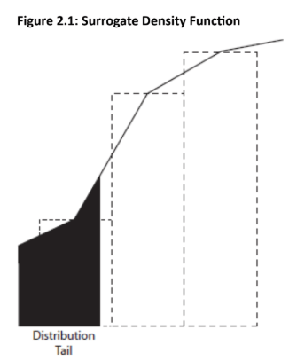
The simplest adjustment involves connecting the midpoints between successive histogram bars (creating a "surrogate density function").
-
Mass Preservation: By connecting the midpoints, the lower bar "receives" area from the upper bar, ensuring that the total area (probability) is conserved, only displaced.
-
-
-
Major Improvement: This allows VaR to be calculated for any confidence level (e.g., 95.5%), offering a major improvement over traditional HS.
-
The linear adjustment is a simple solution to the interval problem. A more complicated adjustment would involve connecting curves, rather than lines, between successive bars to better capture the characteristics of the data.
Topic 3. Applying Nonparametric Estimation
Topic 4. Weighted Historical Simulation Approaches
-
Current Method Assumptions
- Uses current and past n observations up to cutoff point for VaR calculation
- Observations beyond cutoff have zero weight
- Relevant n observations equally weighted at (1/n)
-
Key Problems
- Arbitrary cutoff: nth observation equally important as others, but (n+1)th observation has zero weight
- Ghost effects: Previous events remain in calculation until dropping off after n periods
- Strong independence assumption: Assumes observations are independent and identically distributed (i.i.d.)
- Seasonality issues: Assumption likely violated by data with seasonal volatility
-
Solution: Four improvements to traditional historical simulation method identified:
-
Age-Weighted Historical Simulation
-
Volatility-Weighted Historical Simulation
-
Correlation-Weighted Historical Simulation
-
Filtered Historical Simulation
-
Practice Questions: Q2
Q2. All of the following approaches improve the traditional historical simulation approach for estimating VaR except the:
A. volatility-weighted historical simulation.
B. age-weighted historical simulation.
C. market-weighted historical simulation.
D. correlation-weighted historical simulation.
Practice Questions: Q2 Answer
Explanation: C is correct.
Market-weighted historical simulation is not discussed in this reading. Age- weighted historical simulation weights observations higher when they appear closer to the event date. Volatility-weighted historical simulation adjusts for changing volatility levels in the data. Correlation-weighted historical simulation incorporates anticipated changes in correlation between assets in the portfolio.
Topic 5. Age-Weighted Historical Simulation
-
The fundamental adjustment is to weight recent observations more and distant observations less to reflect the principle that recent market conditions are more relevant for current risk forecasts.
-
Weighting Scheme (Boudoukh, Richardson, and Whitelaw): Assume w(1) is the probability weight for the observation that is one day old. Then w(2) can be defined as λw(1), w(3) can be defined as λ2w(1), and so on.
-
Decay Parameter (λ): Used to control how quickly the weight of an observation decays.
-
The parameter λ can take values 0≤λ≤1.
-
Values close to 1 indicate slow decay (older data retains importance).
-
-
-
Weight:
-
The weight for an observation i days old is:
-
All the weights must sum to 1. This means that
-
-
Special Case: Traditional HS is a special case of age-weighted simulation where λ=1 (i.e., no decay) over the estimation window.
-
Implication: This approach reduces the impact of ghost effects and older, potentially irrelevant events that may not reoccur
Practice Questions: Q3
Q3. Which of the following statements about age-weighting is most accurate?
A. The age-weighting procedure incorporates estimates from GARCH models.
B. If the decay factor in the model is close to 1 , there is persistence within the data set.
C. When using this approach, the weight assigned on day i is equal to
D. The number of observations should at least exceed 250.
Practice Questions: Q3 Answer
Explanation: B is correct.
If the intensity parameter (i.e., decay factor) is close to 1, there will be persistence (i.e., slow decay) in the estimate. The expression for the weight on day i has i in the exponent when it should be n. While a large sample size is generally preferred, some of the data may no longer be representative in a large sample.
Topic 6. Volatility-Weighted Historical Simulation
-
The approach incorporates changing volatility into the risk estimation. The intuition is that:
-
If current volatility has increased, using raw historical data will underestimate current risk.
-
If current volatility has decreased, using raw historical data will overstate current risk.
-
-
Adjustment Procedure: Daily returns, , are adjusted upward or downward based on the current volatility forecast relative to the historical volatility forecast on day t , which is estimated from a GARCH or EWMA model.
-
Volatility-Adjusted Return, :
-
replaces in the data set.
-
VaR Calculation: VaR, ES, and other coherent risk measures are then calculated in the usual way (as in traditional HS), but using the volatility-adjusted returns .
-
-
Advantages
-
Explicitly incorporates volatility into the estimation.
-
Near-term VaR estimates are more sensible in light of current market conditions.
-
Allows for VaR estimates that are higher than the maximum historical loss.
-
Practice Questions: Q4
Q4. Which of the following statements about volatility-weighting is true?
A. Historic returns are adjusted, and the VaR calculation is more complicated.
B. Historic returns are adjusted, and the VaR calculation procedure is the same.
C. Current period returns are adjusted, and the VaR calculation is more complicated.
D. Current period returns are adjusted, and the VaR calculation is the same.
Practice Questions: Q4 Answer
Explanation: B is correct.
The volatility-weighting method adjusts historic returns for current volatility.
Specifically, return at time t is multiplied by (current volatility estimate /
volatility estimate at time t). However, the actual procedure for calculating VaR using a historical simulation method is unchanged; it is only the inputted data that changes.
Topic 7. Correlation-Weighted Historical Simulation
-
This methodology is an extension of volatility-weighting that incorporates updated correlations (covariances) between asset pairs in a portfolio.
-
Methodology Overview
-
Adjustment: The historical variance-covariance (Σ) matrix needs to be adjusted to reflect the current information environment.
-
Intuitively: Historic returns are "multiplied" by the revised correlation matrix to yield updated correlation-adjusted returns.
-
The variance-covariance Matrix
-
-
-
Diagonal Elements: Represent the updated variances of the individual assets (i.e., the volatility adjustments from the previous approach).
-
Off-Diagonal Elements: Represent the updated covariances between asset pairs (i.e., the correlation adjustments).
-
-
-
Correlation- vs. Volatility-Weighting: Correlation-Weighted Simulation is a richer complex and analytical tool than Volatility-Weighted Simulation because it incorporates both: variance adjustments (volatilities) and covariance adjustments (correlations).
Topic 8. Filtered Historical Simulation
-
Overview
- Most comprehensive and complex nonparametric estimator
- Combines historical simulation with conditional volatility models (GARCH, asymmetric GARCH)
- Merges traditional approach attractions with sophisticated volatility modeling
-
Key Features
- Captures conditional volatility and volatility clustering
- Incorporates surprise factor with asymmetric effects on volatility
- Sensitive to changing market conditions
- Can predict losses outside historical range
-
Methodology
- Forecast volatility for each day in sample period
- Standardize volatility by dividing by realized returns
- Use bootstrapping to simulate returns incorporating current volatility
- Identify VaR from simulated distribution
-
Advantages
- Extends to longer holding periods and multi-asset portfolios
- Computationally reasonable even for large portfolios
- Strong empirical support for predictive ability
Topic 9. Advantages of Nonparametric Methods
-
Advantages of nonparametric methods include:
-
Intuitive and often computationally simple (even on a spreadsheet).
-
Not hindered by parametric violations of skewness, fat tails, et cetera.
-
Avoids complex variance-covariance matrices and dimension problems.
-
Data is often readily available and does not require adjustments (e.g., financial statements adjustments).
-
Can accommodate more complex analysis (e.g., by incorporating age-weighting with volatility-weighting).
-
-
Disadvantages of nonparametric methods include:
-
Analysis depends critically on historical data.
-
Volatile data periods lead to VaR and ES estimates that are too high.
-
Quiet data periods lead to VaR and ES estimates that are too low.
-
Difficult to detect structural shifts/regime changes in the data.
-
Cannot accommodate plausible large impact events if they did not occur within the sample period.
-
Difficult to estimate losses significantly larger than the maximum loss within the data set (historical simulation cannot; volatility-weighting can, to some degree).
-
Need sufficient data, which may not be possible for new instruments or markets.
-
Topic 10. Disadvantages of Nonparametric Methods
Practice Questions: Q5
Q5. All of the following items are generally considered advantages of nonparametric estimation methods except:
A. ability to accommodate skewed data.
B. availability of data.
C. use of historical data.
D. little or no reliance on covariance matrices.
Practice Questions: Q5 Answer
Explanation: C is correct.
The use of historical data in nonparametric analysis is a disadvantage, not an
advantage. If the estimation period was quiet (volatile) then the estimated risk measures may understate (overstate) the current risk level. Generally, the largest VaR cannot exceed the largest loss in the historical period. On the other hand, the remaining choices are all considered advantages of nonparametric methods. For instance, the nonparametric nature of the analysis can accommodate skewed data, data points are readily available, and there is no requirement for estimates of covariance matrices.