Book 2. Credit Risk

FRM Part 2

CR 11. Portfolio Credit Risk

Presented by: Sudhanshu

Module 1. Credit Portfolios and Credit VaR

Module 2. Conditional Default Probabilities and Credit VaR with Copulas

Module 1. Credit Portfolios and Credit VaR

Topic 1. Default Correlation for Credit Portfolios

Topic 2. Credit Portfolio Framework

Topic 3. Credit VaR

Topic 1. Default Correlation for Credit Portfolios

Credit Risks: When analyzing credit portfolios, you need to consider various risks like default probability, loss given default (LGD), risk of deteriorating credit ratings, spread risk, and loss from bankruptcy restructuring.
Default Correlation: Measures the probability of multiple defaults occurring within a credit portfolio consisting of multiple obligors.
Modeling with Bernoulli Variables: Default correlation can be modeled using the outcomes of Bernoulli-distributed random variable
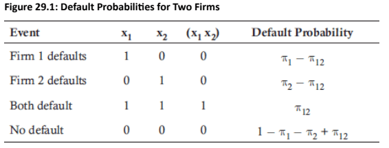
- Suppose there are two firms whose probabilities of default over the next time horizon t are and for each firm, respectively. In addition, there is a joint probability that both firms will default over time horizon t equal to .
- Fig 29.1 illustrates the four possible random outcomes where 0 denotes the event of no default and 1 denotes default.

\pi_1

\pi_2

\pi_{12}

\pi_1

x_i

Topic 1. Default Correlation for Credit Portfolios

Key Statistical Components:
- Mean ( ): The expected value for each firm is its individual probability of default ( ).
- Expected Joint Default: .
- Variance: Computed as
- Covariance: Computed as
Default Correlation Formula: The default correlation ( ) is defined as the covariance of the two firms divided by the product of their standard deviations:
3. Example: Calculating Default Correlation
- Firm 1 (BBB+):
- Firm 2 (BBB):
- Joint Default Probability:

E[x_1x_2]=\pi_{12}

\pi_i

\pi_i(1-\pi_i).

E[x_i]

\pi_{12}-\pi_1 \pi_2.

\rho_{12}

\rho_{12} = \frac{\pi_{12} - \pi_1\pi_2}{\sqrt{\pi_1(1 - \pi_1)}\sqrt{\pi_2(1 - \pi_2)}}

\pi_1 = 0.002

\pi_2 = 0.003

\pi_{12} = 0.00015

Topic 1. Default Correlation for Credit Portfolios

Solution:
- Default correlation can be calculated using the following formula for a two-credit portfolio:

\begin{aligned} \rho_{12} & =\frac{\pi_{12}-\pi_1 \pi_2}{\sqrt{\pi_1\left(1-\pi_1\right)} \sqrt{\pi_2\left(1-\pi_2\right)}}=\frac{0.00015-(0.002 \times 0.003)}{\sqrt{0.002(1-0.002)} \sqrt{0.003(1-0.003)}} \\ & =\frac{0.000144}{\sqrt{0.001996} \sqrt{0.002991}}=\frac{0.000144}{(0.04468 \times 0.05469)} \\ & =0.0589 \text { or } 5.89 \% \end{aligned}

Practice Questions: Q1

Q1. Which of the following equations best defines the default correlation for a two-firm credit portfolio?

\rho_{12}=\frac{\pi_{12}-\pi_1 \pi_2}{\sqrt{\pi_1 (1-\pi_1)}\sqrt{\pi_2(1-\pi_2)}}

\rho_{12}=\frac{\pi_{12}}{\sqrt{\pi_1 (1-\pi_1)}\sqrt{\pi_2(1-\pi_2)}}

\rho_{12}=\frac{\pi_{12}}{\sqrt{(1-\pi_1)}\sqrt{(1-\pi_2)}}

\rho_{12}=\frac{\pi_{12}-\pi_1 \pi_2}{\sqrt{\pi_1 }\sqrt{\pi_2}}

Practice Questions: Q1 Answer

Explanation: A is correct.

The default correlation for a two-firm credit portfolio is defined as:

\rho_{12}=\frac{\pi_{12}-\pi_1 \pi_2}{\sqrt{\pi_1 (1-\pi_1)}\sqrt{\pi_2(1-\pi_2)}}

Topic 2. Credit Portfolio Framework

There are several drawbacks in using correlation-based credit portfolio framework:
- Computational Complexity: The number of required calculations grows exponentially with portfolio size
  - Three-firm framework requires 8 event outcomes (2³) with only 7 conditions
  - Ten-firm portfolio generates 1,024 event outcomes (2¹⁰) with 56 conditions
  - Pairwise correlations equal n(n-1), often simplified to a nonnegative parameter
- Limited Applicability to Complex Instruments: Certain credit positions do not fit well within the simplistic framework
  - Guarantees, revolving credit agreements, and contingent liabilities have option-like features not captured by the model
  - CDS basis trades driven by technical factors (e.g., liquidity constraints during subprime crisis) rather than purely credit or market risk
  - Convertible bonds exhibit characteristics of both credit and equity portfolios influenced by multiple risk factors
- Data Limitations and Estimation Issues: Sparse default data creates significant estimation challenges
  - Firm defaults are rare events, causing estimated correlations to vary greatly by time horizon and industry
  - Most studies use an estimated correlation of approximately 0.05
  - Default correlations are small in magnitude, making joint default probabilities even smaller and harder to estimate reliably

(2^n)

Practice Questions: Q2

Q2. Suppose a portfolio manager is using a default correlation framework for measuring credit portfolio risk. How many unique event outcomes are there for a credit portfolio with eight different firms?

A. 10.

B. 56.

C. 256.

D. 517.

Practice Questions: Q2 Answer

Explanation: C is correct.

There are 256 event outcomes for a credit portfolio with eight different firms calculated as: .

2^8=256

Topic 3. Credit VaR

Credit Value at Risk (Credit VaR): Measures the potential loss in a credit portfolio over a specific time horizon at a given confidence level.
Definition and Core Concepts
- Credit VaR Formula: It is defined as the quantile of the credit loss minus the expected loss of the portfolio.
- Impact of Default Correlation: Correlation does not change the expected loss; instead, it impacts the volatility and the extreme quantiles (the tail) of the loss distribution.
  - Default Correlation = 1: The portfolio provides no diversification benefits and behaves as if there were only one credit position.
  - Default Correlation = 0: The portfolio acts as a binomial-distributed random variable because individual defaults are independent.
- Impact of Granularity: Granularity refers to reducing the weight of each individual credit by increasing the total number of credits in the portfolio.
  - Inverse Relationship: As a credit portfolio becomes more granular (higher $n$ ), the Credit VaR decreases.
  - Low Default Probability: when the default probability is low, the credit VaR is not impacted as much when the portfolio becomes more granular.

Topic 3. Credit VaR

Example 1: Computing credit VaR (default correlation = 1, number of credits = n). Suppose there is a portfolio with a value of $1,000,000 that has n credits. Each of the credits has a default probability of π percent and a recovery rate of zero. This implies that in the event of default, the position has no value and is a total loss. What is the extreme loss given default and credit VaR at the 95% confidence level if π is 2% and the default correlation is equal to 1?
Answer: With the default correlation equal to 1, the portfolio will act as if there is only one credit. Viewing the portfolio as a binomial-distributed random variable, there are only two possible outcomes for a portfolio acting as one credit. Regardless of whether the number of credits in the portfolio, n, is 1, 20, or 1,000, it will still act as one credit when the correlation is 1.

The portfolio has a π percent probability of total loss and a (1 − π) percent probability of zero loss. Therefore, with a recovery rate of zero, the extreme LGD is $1,000,000. The expected loss is equal to the portfolio value times π and is $20,000 in this example (= 0.02*$1,000,000). There is a 98% probability that the loss will be 0, given the fact that π equals 2%. The credit VaR is defined as the quantile of the credit loss minus the expected loss of the portfolio. Therefore, at the 95% confidence level, the credit VaR is equal to −$20,000 (= 0 - expected loss of $20,000).
Note that if π was greater than (1 − confidence level), the credit VaR would have

been calculated as $1,000,000 − $20,000 = $980,000.

Topic 3. Credit VaR

Example 2: Computing credit VaR (default correlation = 0, number of credits = 50). Again suppose there is a $1,000,000 portfolio with n credits that each have a default probability of π percent and a zero recovery rate. However, in this example the default correlation is 0, n = 50, and π = 0.02. In addition, each credit is equally weighted and has a terminal value of $20,000 if there is no default. The number of defaults is binomially distributed with parameters of n = 50 and π = 0.02. The 95th percentile of the number of defaults based on this distribution is 3.What is the credit VaR at the 95% confidence level based on these parameters?
Answer: The expected loss in this case is also $20,000 (= $1,000,000 X 0.02). If there are three defaults, the credit loss is $60,000 (= 3 X $20,000). The credit VaR at the 95% confidence level is $40,000 (= credit loss of $60,000 - expected loss of $20,000).

Topic 3. Credit VaR

Example 3: Computing credit VaR (default correlation = 0, number of credits = 1,000). Suppose there is a $1,000,000 portfolio with n credits that each have a default probability, π, equal to 2% and a zero recovery rate. The default correlation is 0 and n = 1,000. There is a probability of 28 defaults at the 95th percentile based on the binomial distribution with the parameters of n = 1,000 and π = 0.02. What is the credit VaR at the 95% confidence level based on these parameters?
Answer: The 95th percentile of the credit loss distribution is $28,000 [= 28 X ($1,000,000/1,000)]. The expected loss in this case is $20,000 (= $1,000,000 X 0.02). The credit VaR is then $8,000 (= $28,000 − expected loss of $20,000). Thus, as the credit portfolio becomes more granular, the credit VaR decreases. For very large credit portfolios with a large number of independent credit positions, the probability that the credit loss equals the expected loss eventually converges to 100%.

Practice Questions: Q3

Q3. Suppose a portfolio has a notional value of $1,000,000 with 20 credit positions. Each of the credits has a default probability of 2% and a recovery rate of zero. Each credit position in the portfolio is an obligation from the same obligor, and therefore, the credit portfolio has a default correlation equal to 1. What is the credit value at risk at the 99% confidence level for this credit portfolio?

A. $0.

B. $1,000.

C. $20,000.

D. $980,000

Practice Questions: Q3 Answer

Explanation: D is correct.

With the default correlation equal to 1, the portfolio will act as if there is only one credit. Viewing the portfolio as a binomial distributed random variable, there are only two possible outcomes for a portfolio acting as one credit. The portfolio has a 2% probability of total loss and a 98% probability of zero loss. Therefore, with a
recovery rate of zero, the extreme loss given default is $1,000,000. The expected loss is equal to the portfolio value times π and is $20,000 in this example (0.02 × $1,000,000). The credit VaR is defiined as the quantile of the credit loss less the expected loss of the portfolio. At the 99% confiidence level, the credit VaR is equal to $980,000 ($1,000,000 minus the expected loss of $20,000).

Module 2. Conditional Default Probabilities And Credit VaR with Copulas

Topic 1. Conditional Default Probabilities

Topic 2. Conditional Default Distribution Variance

Topic 3. Credit VaR With a Single-Factor Model

Topic 4. Credit VaR With Simulation

Topic 1. Conditional Default Probabilities

Single-Factor Model: Used to examine how default correlations vary based on a credit position's sensitivity to the market, known as its beta).
Single-Factor Model Framework: The model assumes that an individual firm’s asset return ( ) is driven by a common market factor ( $m$ ) and a unique idiosyncratic shock ( ):
- where
  - : : firm's standard deviation of idiosyncratic risk
  - : firm's idiosyncratic shock
The Default Condition:
- Assumption: Each (error term) is not correlated with other credits, making each return on asset ( ) a standard normal variate
- Pairwise Correlation Structure: The correlation between individual asset returns for any two firms i and j equals
- A firm is assumed to default if its asset return ( ) falls below a specific threshold ( ), which represents the logarithmic distance to the defaulted asset value measured in standard deviations.
  - Firm defaults if

a_i=\beta_i m+\sqrt{1-\beta_i^2 \varepsilon_i}

\varepsilon_i

\sqrt{1-\beta_i^2}

\varepsilon_i

a_i

a_{\mathrm{i}} \leq k_{\mathrm{i}}

a_{\mathrm{i}}

k_{\mathrm{i}}

a_{\mathrm{i}}

\varepsilon_i

\beta_{\mathrm{i}} \beta_{\mathrm{i}}

Topic 1. Conditional Default Probabilities

Conditional Independence: Conditional independence states that once the market factor is realized, the default risks of individual firms become independent of one another.
- This is because the model assumes asset risk and returns are correlated only with the market factor.
- Conditional independence property makes the single-factor model useful in estimating portfolio credit risk.
Impact of Market Conditions on Default: To measure dafault probabilities conditional on market movements or economic health, we make some adjustments in the model.
Conditional Default Probabilitity: By substituting a specific market factor value ( ), into the single-factor model and rearranging, we get:
- Default Risk: Measured by the distance to default, , has only one random variable which is
- Impact of Conditioning: Conditioning on a specific market value shifts the default distribution's mean based on beta ( ), while the default threshold ( ) remains unchanged but the standard deviation reduces from 1 to

\sqrt{1-\beta_i^2}

\varepsilon_i

\beta_i > 0

\overline{m}

\mathrm{a}_{\mathrm{i}}-\beta_{\mathrm{i}} \overline{\mathrm{~m}}=\sqrt{1-\beta_1^2} \varepsilon_i

k_i

\mathrm{a}_{\mathrm{i}}-\beta_{\mathrm{i}} \overline{\mathrm{~m}}

\beta_i \overline{m}

Topic 1. Conditional Default Probabilities

Specifying a specific value for the market parameter, m, in the single-factor model results in the following implications
- The conditional probability of default will be greater or smaller than the unconditional probability of default as long as or are not equal to zero. This reduces the default triggers or number of idiosyncratic shocks, , so that it is less than or equal to . As the market factor goes from strong to weak economies, a smaller idiosyncratic shock will trigger default.
- The conditional standard deviation is less than the unconditional standard deviation of 1.
- Individual asset returns, , and idiosyncratic shocks, , are independent from other firms’ shocks and returns.

\overline{m}

\beta_i

\varepsilon_i

\mathrm{k}_{\mathrm{i}}-\beta_{\mathrm{i}} \overline{\mathrm{~m}}

\sqrt{1-\beta_i^2}

a_i

\varepsilon_i

Topic 2. Conditional Default Distribution Variance

Conditional Cumulative Default Probability Function: The conditional cumulative default probability function:
- Mean: New distance of default based on the realized market factor,
- Variance: Assumes conditional independence,
Interpretation: Given a realized market factor, , the probability of default is based on the distance of the new default trigger of idiosyncratic shocks, , measured in standard deviations below its mean of zero.
Special Case: If we assume that distribution parameters (β, k, and π) are equal for all firms, then the probability of a joint default for two firms is given by:
- In this case, pairwise default correlation can be written as:

p(m)=\Phi\left(\frac{k_i-\beta_i \bar{m}}{\sqrt{1-\beta_i^2}}\right)

\text{Variance}=\sqrt{1-\beta_i^2}

\text{Mean}=\beta_{\mathrm{i}} \overline{m}

\overline{m}

\varepsilon_i

\Phi\binom{k}{k}=\mathrm{P}[-\infty \leq \mathrm{a} \leq \mathrm{k},-\infty \leq \mathrm{a} \leq \mathrm{k}]

\rho=\frac{\Phi\binom{k}{k}-\pi^2}{\pi(1-\pi)}

Practice Questions: Q1

Q1. A portfolio manager uses the single-factor model to estimate default risk. What is the mean and standard deviation for the conditional distribution when a specific realized market value is used?

A. The mean and standard deviation are equivalent in the standard normal distribution.

B. The mean is and the standard deviation is .

C. The mean is and the standard deviation is .

D. The mean is and the standard deviation is 1.

\bar{m}

\beta_i \overline{m}

\sqrt{1-\beta_i^2}

\bar{m}

\beta_i

Practice Questions: Q1 Answer

Explanation: B is correct.

The conditional distribution is a normal distribution with a mean of and a standard deviation of

\sqrt{1-\beta_i^2}

\beta_i \overline{m}

Topic 3. Credit VaR with a Single-Factor Model

Binary Default Outcomes: In previous model, credit loss distributions were estimated for extreme default correlations of 0 or 1.
Distribution of Loss Severity: To determine the distribution of loss severity for values between these two extremes, the single-factor model is used to calculate the unconditional probability of a default loss level.
Unconditional Distribution Framework: The unconditional probability of a default loss level is equal to the probability that the realized market return results in a default loss.
- Framework: The individual credit asset returns ( ) are strictly a function of the market return ( $m$ ) and the asset's correlation to the market ( ).
- Credit VaR: The unconditional distribution used to calculate Credit VaR is determined through a systematic four-step process, shown in next slide.
Note: The parameters play an important role in determining the unconditional loss distribution.
- The probability of default, π, determines the unconditional expected default value for the credit portfolio.
- The credit position’s correlation to the market, β, determines the dispersion of the defaults based on the range of the market factor.

a_i

\beta_i

Topic 3. Credit VaR with a Single-Factor Model

Credit VaR Calculation: The unconditional distribution used to calculate Credit VaR is determined through a systematic four-step process.
- Define the Loss Level: The default loss level is treated as a random variable $X$ with realized values $x$ . In this framework, $x$ is not simulated.
- Determine the Market Factor ( $m$ ): For a given loss level $x$ , the value for the market factor is determined at the probability of that stated loss level. The relationship is expressed as:
  - To find the specific market factor return ( ) for a given loss level ( ), the relationship is inverted:
- Standard Normal Assumption: The market factor is assumed to follow a standard normal distribution. Consequently, a loss level at a 99% confidence level (0.01 probability) corresponds to a value of $-2.33$ on the standard normal distribution.
- Aggregation: These steps are repeated for every individual credit in the portfolio to establish the complete loss probability distribution.

x(m) = p(m) = \Phi\left(\frac{k - \beta \bar{m}}{\sqrt{1 - \beta^2}}\right)

\bar{m}

\bar{x}

\Phi^{-1}(\bar{x}) = \left(\frac{k - \beta \bar{m}}{\sqrt{1 - \beta^2}}\right)

Topic 3. Credit VaR with a Single-Factor Model

Example: Suppose a credit position has a correlation to the market factor of 0.25. What is the realized market value used to compute the probability of reaching a default threshold at the 99% confidence level?
Answer: At the 99% confidence level, the default loss level has a default probability, π, of 0.01. A default loss level of 0.01 corresponds to –2.33 on the standard normal distribution. The relationship between the default loss level and the given market return, , is defined by:
- The realized market value is computed as follows:
- The probability that the default threshold is reached is the same probability that the realized market return is −0.296 or lower.

\begin{aligned} & -2.33=\frac{-2.33-(0.25) \overline{\mathrm{m}}}{\sqrt{1-0.25^2}} \\ & -2.33(0.9682)=-2.33-(0.25) \overline{\mathrm{m}} \\ & -2.256+2.33=-(0.25) \overline{\mathrm{m}} \\ & 0.074=-(0.25) \overline{\mathrm{m}} \implies \overline{\mathrm{m}} = -0.296\\ \end{aligned}

\bar{m}

\begin{aligned} p(\bar{m})=0.01&=\Phi\left(\frac{k-\beta \bar{m}}{\sqrt{1-\beta^2}}\right) \implies \Phi^{-1}(0.01) \approx-2.33&=\left(\frac{\mathrm{k}-\beta \overline{\mathrm{m}}}{\sqrt{1-\beta^2}}\right) \end{aligned}

Practice Questions: Q2

Q2. Suppose a credit position has a correlation to the market factor of 0.5. What is the realized market value that is used to compute the probability of reaching a default threshold at the 99% confidence level?

A. −0.2500.

B. −0.4356.

C. −0.5825.

D. −0.6243.

Practice Questions: Q2 Answer

Explanation: D is correct.

A default loss level of 0.01 corresponds to −2.33 on the standard normal distribution. The realized market value is computed as follows:

\begin{aligned} & -2.33=\frac{-2.33-(0.5) \overline{\mathrm{m}}}{\sqrt{1-0.5^2}} \\ & -2.33(0.86603)=-2.33-(0.5) \overline{\mathrm{m}} \\ & -2.01785+2.33=-(0.5) \overline{\mathrm{m}} \\ & 0.31215=-(0.5) \\ & -0.62430=\overline{\mathrm{m}} \end{aligned}

Topic 4. Credit VaR with Simulation

Simulated Results using Copulas: Copulas offer a mathematical framework for determining how defaults are correlated within a portfolio using simulated results.
Copula Methodology: The following four steps are used to compute a credit VaR under the copula methodology:
- Step 1: Define the copula function: Establish the mathematical dependency structure between the credits.
- Step 2: Simulate default times: Generate random variables representing default times for each credit in the portfolio.
- Step 3: Obtain market values and P&L: Use the simulated default times to determine the market values and profit and loss (P&L) data for each specific scenario.
- Step 4: Compute portfolio statistics: Aggregate the simulated terminal value results to derive the portfolio's distribution statistics.

Topic 4. Credit VaR with Simulation

Example: Suppose there is a credit portfolio with two loans (rated CCC and BB) that each has a notional value of $1,000,000. Fig 29.2 shows four possible outcomes over a default time horizon of 1 year for this credit portfolio. The four event outcomes are only the BB rated loan defaults, only the CCC rated loan defaults, both loans default, or no loans default. How can credit VaR be estimated for this portfolio assuming a correlation of 0.25?
Answer: The credit VaR is estimated using the copula approach by following below steps:
- Simulate 1,000 values using a copula function. The most common copula used to calculate credit VaR is the normal copula.
- The 2,000 simulated values (1,000 pair simulations results in 2,000 values) are then mapped to their standard univariate normal quantile which results in 1,000 pairs of probability values.
- The first and second elements of each probability pair are mapped to the BB and CCC default times, respectively.
- A terminal value is assigned to each loan for each simulation. The values are added up for the two loans, and the sum of the no-default event value is subtracted to determine the loss. Fig 29.3 shows the sum of the terminal values and losses for 1,000 simulations.

\begin{array}{lc} \hline \text {Fig 49.2 } & \\ \hline \text { Event } & \text { Default Time } \\ \hline \text { BB default } & \left(\tau_{\mathrm{BB}, \mathrm{i}} \leq 1, \tau_{\mathrm{CCC}, \mathrm{i}}>1\right) \\ \text { CCC default } & \left(\tau_{\mathrm{BB}, \mathrm{i}}>1, \tau_{\mathrm{CCC}, \mathrm{i}} \leq 1\right) \\ \text { Both default } & \left(\tau_{\mathrm{BB}, \mathrm{i}} \leq 1, \tau_{\mathrm{CCC}, \mathrm{i}} \leq 1\right) \\ \text { No default } & \left(\tau_{\mathrm{BB}, \mathrm{i}}>1, \tau_{\mathrm{CCC}, \mathrm{i}}>1\right) \\ \hline \end{array}

\begin{array}{lc} \hline \text {Fig 49.3 } & \\ \hline \text{Event} & \text{Default Time} & \text{Terminal Value} & \text{Loss} \\ \hline \text{BB default} & (\tau_{\mathrm{BB},i} \le 1,\ \tau_{\mathrm{CCC},i} > 1) & 1{,}480{,}000 & 710{,}000 \\ \text{CCC default} & (\tau_{\mathrm{BB},i} > 1,\ \tau_{\mathrm{CCC},i} \le 1) & 1{,}410{,}000 & 780{,}000 \\ \text{Both default} & (\tau_{\mathrm{BB},i} \le 1,\ \tau_{\mathrm{CCC},i} \le 1) & 700{,}000 & 1{,}490{,}000 \\ \text{No default} & (\tau_{\mathrm{BB},i} > 1,\ \tau_{\mathrm{CCC},i} > 1) & 2{,}190{,}000 & 0 \\ \hline \end{array}

Topic 4. Credit VaR with Simulation

The loss level sums from the simulation are then used to determine the credit VaR based on the simulated distribution. In this simulation, the 99% confidence level corresponds to the $1,490,000 loss where both loans default.
The 95% confidence level corresponds to the $780,000 value because the lower 5% of the simulated values resulted in defaults with a total loss of $780,000.