Perform Customer Segmentation Using Clustering

Business Scenario
Welcome back!
Today is your eighth day as a Junior Data Scientist on the Telecom Customer Intelligence Project
The analytics team has successfully developed customer churn prediction models. Management now wants to understand customer behavior by identifying groups of customers with similar characteristics and usage patterns.
Since the objective is to discover hidden patterns without a target variable, you will use Unsupervised Learning techniques. In this lab, you will apply K-Means Clustering and Hierarchical Clustering to perform customer segmentation and generate business insights.

As part of this project, you will:
- Understand Unsupervised Learning.
- Understand Customer Segmentation.
- Apply K-Means Clustering.
- Apply Hierarchical Clustering.
- Identify customer segments.
- Interpret clustering results for business decision-making.
Pre-Lab Preparation
Topic : Unsupervised Learning
1) Clustering-based Customer Segmentation (K-Means, Hierarchical Clustering)
git pull origin branchName
Git Pull
Task 1: Perform Customer Segmentation Using K-Means Clustering
Before building a clustering model, it is important to understand how customer segmentation works using Unsupervised Learning.

Unsupervised Learning
Unsupervised Learning is a type of Machine Learning where the model learns patterns from unlabeled data. Unlike supervised learning, there is no target variable or predefined output. The algorithm analyzes the data and identifies hidden structures, relationships, or groups on its own.
Common Algorithms:
- K-Means Clustering
- Hierarchical Clustering
- DBSCAN
- Principal Component Analysis (PCA)
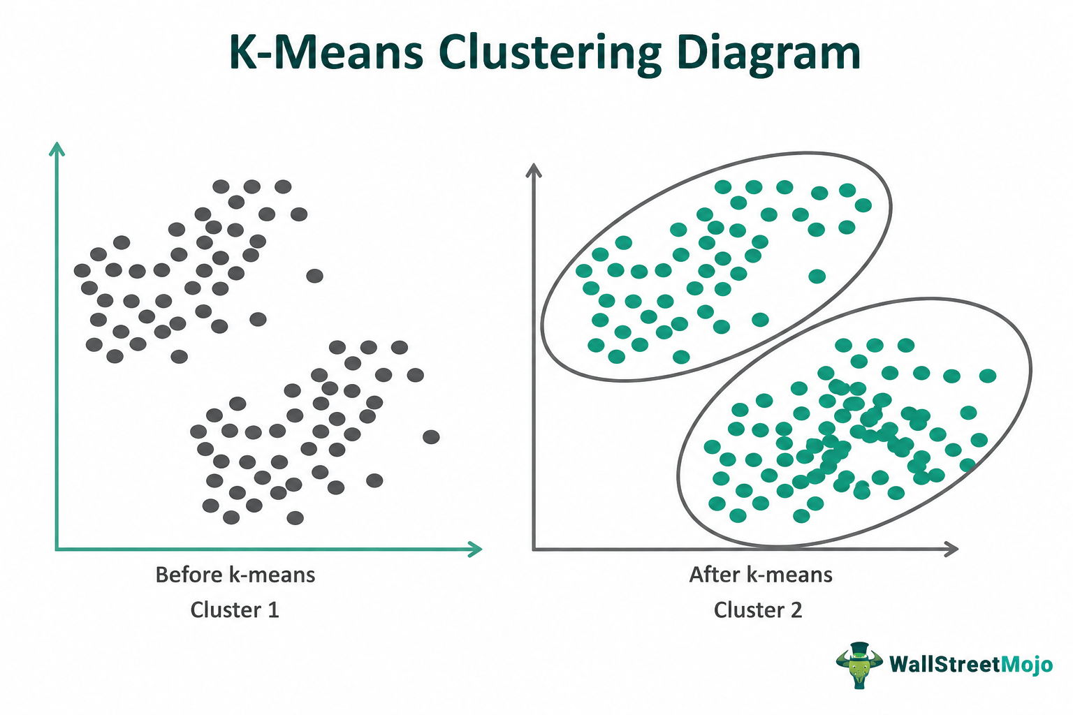
K-Means Clustering
K-Means Clustering is a popular unsupervised learning algorithm used to group similar data points into K clusters.
The goal is to create clusters where data points within the same group are more similar to each other than to those in other groups.
The algorithm starts by selecting the number of clusters (K) and initializing K centroids. Each data point is assigned to the nearest centroid, and the centroids are then updated based on the mean of the assigned points. This process is repeated until the clusters become stable.
K-Means is widely used for customer segmentation, market analysis, and pattern discovery. It is simple, efficient, and works well with large datasets, but it requires the value of K to be specified beforehand and can be affected by outliers.
Elbow Method
The Elbow Method helps determine the optimal number of clusters.
It calculates the Sum of Squared Errors (SSE) for multiple cluster values.
The point where the curve starts flattening is considered the optimal cluster count.
Import Required Libraries
1
import numpy as np
import pandas as pd
import matplotlib.pyplot as plt
import seaborn as sns
import warnings

warnings.filterwarnings('ignore')
Load and explore dataset
2
df = pd.read_csv("mall.csv")

df.head()
df.shape
df.dtypes
df.duplicated().sum()
df.drop_duplicates(inplace=True)
df.shape
Click to download previous file : ML Lab 13.ipynb
Click to download Dataset : Mall.csv
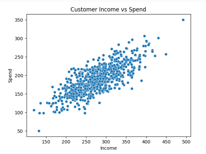
Visualize Customer Distribution
3
sns.scatterplot(x=X1, y=X2)

plt.xlabel("Income")
plt.ylabel("Spend")
plt.title("Customer Income vs Spend")
plt.show()
Scale the Features
4
df_copy = df.copy()

from sklearn.preprocessing import StandardScaler

ss = StandardScaler()

df = ss.fit_transform(df)
Determine the Optimal Number of Clusters
5
from sklearn.cluster import KMeans

SSE = []
K_cluster = []

for k in range(1,21):

    km = KMeans(n_clusters=k)

    km.fit(df)
    SSE.append(km.inertia_)
    K_cluster.append(k)
dict = {
'Value Of K': K_cluster,
'SSE': SSE
}
df1 = pd.DataFrame(dict)
df1sns.scatterplot(
data=df1,
x='Value Of K',
y='SSE'
)
sns.lineplot(
data=df1,
x='Value Of K',
y='SSE',
color='green'
)plt.xlabel('Value of K')
plt.ylabel('Sum of Squared Error')
plt.xticks(df1['Value Of K'])
plt.show()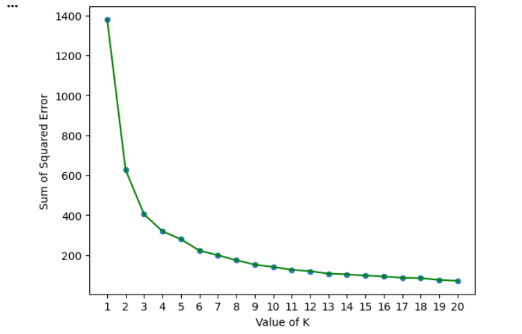
Build the K-Means Model
6
km = KMeans(
    n_clusters=5,
    random_state=1
)
Y_pred = km.fit_predict(df)
Y_pred
Create Customer Segments
7
df_copy['Target'] = Y_pred

df_copy.head()
df_0 = df_copy[df_copy['Target'] == 0]
df_1 = df_copy[df_copy['Target'] == 1]
df_2 = df_copy[df_copy['Target'] == 2]
df_3 = df_copy[df_copy['Target'] == 3]
df_4 = df_copy[df_copy['Target'] == 4]
df_0.shape, df_1.shape, df_2.shape, df_3.shape, df_4.shape
Analyze Cluster Centroids
8
km.cluster_centers_
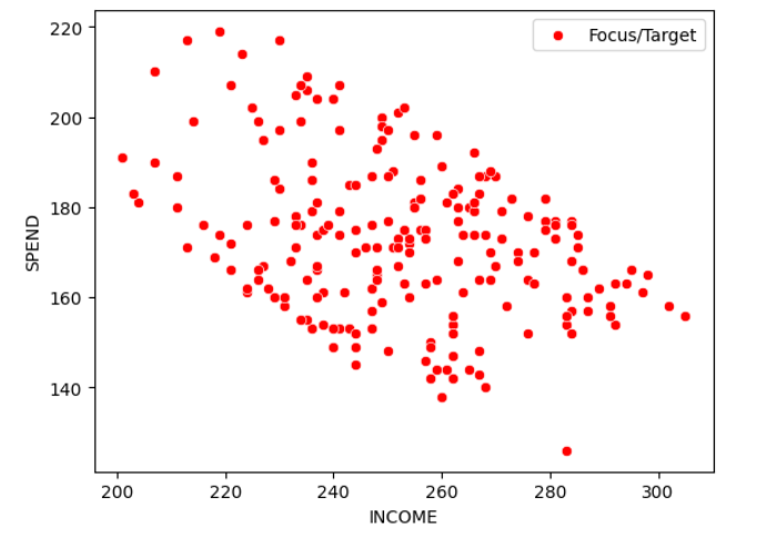
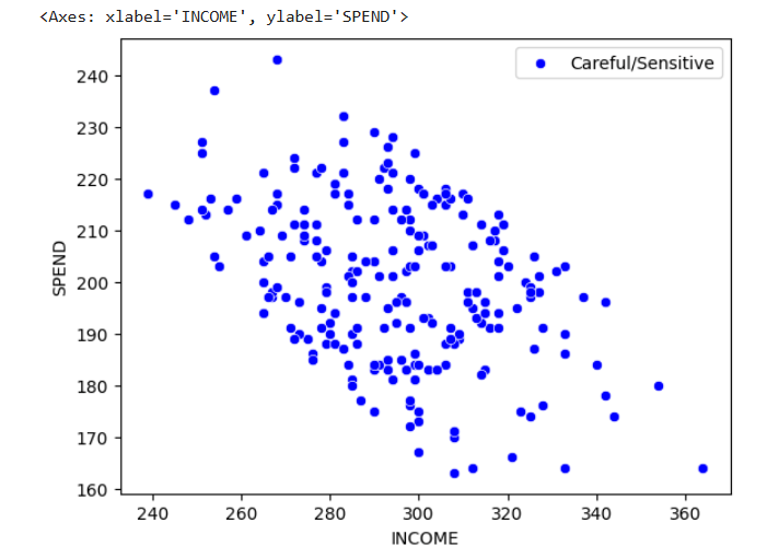
ss.inverse_transform(km.cluster_centers_)Visualize Customer Segments
9
sns.scatterplot(
    data=df_0,
    x="INCOME",
    y="SPEND",
    color="red",
    label="Focus/Target"
)
sns.scatterplot(
    data=df_1,
    x="INCOME",
    y="SPEND",
    color="blue",
    label="Careful/Sensitive"
)
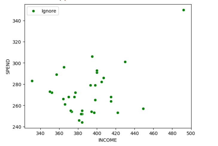
sns.scatterplot(
    data=df_2,
    x="INCOME",
    y="SPEND",
    color="green",
    label="Ignore"
)
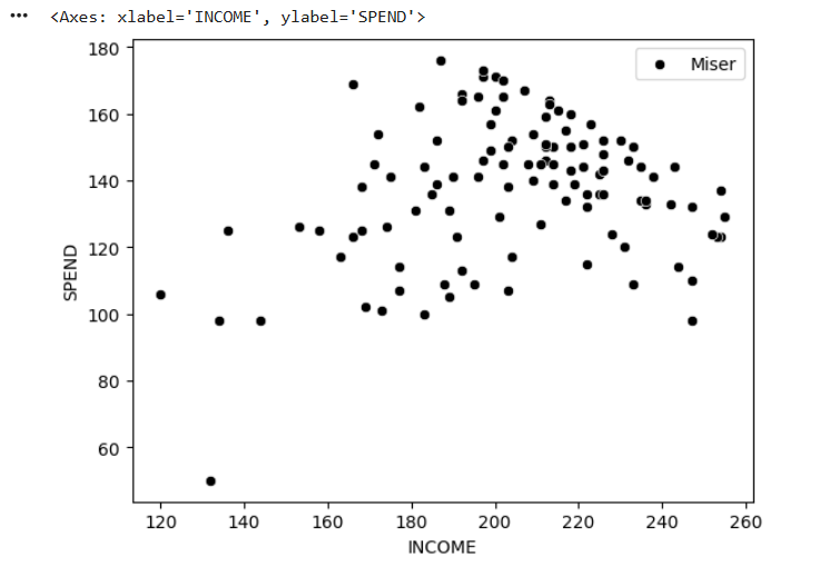
sns.scatterplot(
    data=df_3,
    x="INCOME",
    y="SPEND",
    color="black",
    label="Miser"
)
sns.scatterplot(
    data=df_4,
    x="INCOME",
    y="SPEND",
    color="yellow",
    label="Careless/Target"
)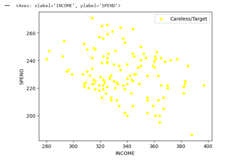
plt.scatter(
    ss.inverse_transform(km.cluster_centers_)[:,0],
    ss.inverse_transform(km.cluster_centers_)[:,1],
    color="purple",
    marker="*",
    s=150
)

plt.show()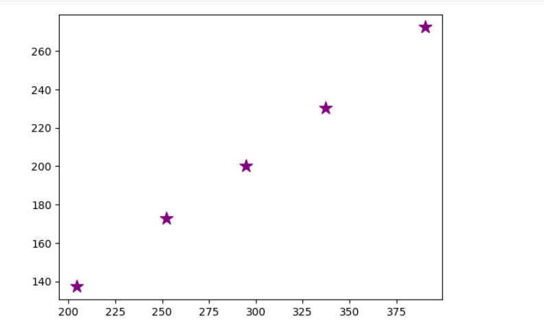
Task 2: Perform Customer Segmentation Using Hierarchical Clustering
While K-Means requires the number of clusters to be specified beforehand, Hierarchical Clustering provides a visual representation of how clusters are formed using a Dendrogram.
Hierarchical Clustering
Hierarchical Clustering creates clusters by building a hierarchy of observations based on similarity.
Unlike K-Means, it does not require the number of clusters to be specified initially.
Types of Hierarchical Clustering
Agglomerative Clustering (Bottom-Up)
- Starts with each observation as an individual cluster.
- Merges similar clusters step-by-step.
Divisive Clustering (Top-Down)
- Starts with one large cluster.
- Divides it into smaller clusters.
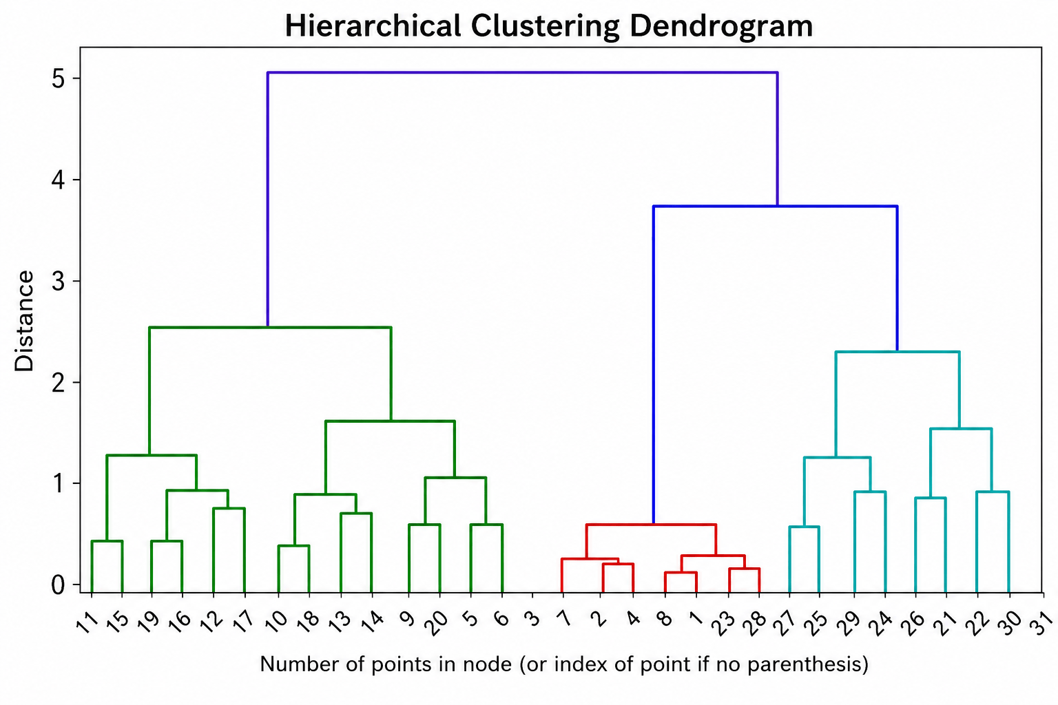
Dendrogram
A Dendrogram is a tree-like diagram used to visualize the clustering process.
It helps identify:
- Cluster similarity
- Cluster formation
- Optimal cluster count
Import Required Libraries
1
from scipy.cluster.hierarchy import dendrogram, linkage
from sklearn.cluster import AgglomerativeClustering
import matplotlib.pyplot as plt
import seaborn as sns
Prepare the Dataset
2
from sklearn.preprocessing import StandardScaler

ss = StandardScaler()

df_scaled = ss.fit_transform(df)
Generate a Dendrogram
3
linked = linkage(
    df_scaled,
    method='ward'
)

plt.figure(figsize=(12,6))

dendrogram(linked)

plt.title("Dendrogram")
plt.xlabel("Customers")
plt.ylabel("Euclidean Distance")

plt.show()
Build the Hierarchical Clustering Model
4
hc = AgglomerativeClustering(
    n_clusters=5
)

y_pred = hc.fit_predict(df_scaled)
y_pred
Create Customer Segments
5
df_copy['Target'] = y_pred

df_copy.head()
df_h0 = df_copy[df_copy['Target'] == 0]
df_h1 = df_copy[df_copy['Target'] == 1]
df_h2 = df_copy[df_copy['Target'] == 2]
df_h3 = df_copy[df_copy['Target'] == 3]
df_h4 = df_copy[df_copy['Target'] == 4]
df_h0.shape, df_h1.shape, df_h2.shape, df_h3.shape, df_h4.shape
Visualize Hierarchical Clusters
6
sns.scatterplot(
    data=df_copy,
    x='INCOME',
    y='SPEND',
    hue='Target',
    palette='Set1'
)
plt.title("Hierarchical Clustering")
plt.show()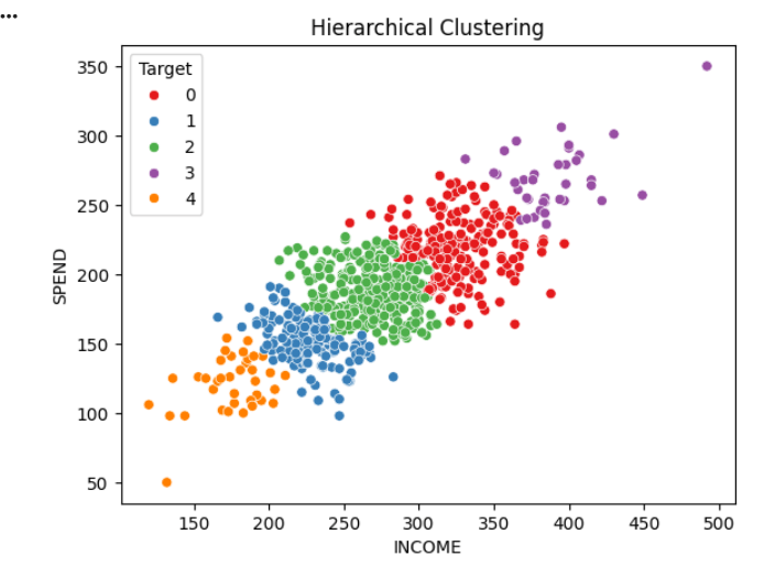
Great job!
You have successfully completed Day 14: Perform Customer Segmentation Using Clustering.
In this lab, you understood Unsupervised Learning and Customer Segmentation, applied K-Means Clustering and the Elbow Method, created customer segments, performed Hierarchical Clustering, generated and interpreted a Dendrogram, built an Agglomerative Clustering model, and compared the results of both clustering techniques for business decision-making.
Checkpoint
You are now ready to Reduce Dimensions Using PCA for Better Insights and simplify complex datasets for analysis.
Next-Lab Preparation
Git Push
git push origin branchNameTopic : Unsupervised Learning
1) PCA