Merging and Retrieving Data Using Lookup Functions

Business Scenario
Welcome!
Today, we received a real project from a client.
The client requires a single interactive dashboard to monitor overall performance, key metrics, and trends in real time.

Pre-Lab Preparation
Topic : Merging and Retrieving Data Using Lookup Functions:
1) Merge the data using lookup functions.
2) Reports that can be filtered by region or product.
git pull origin branchName
Git Pull
Task 1: Merge the data using lookup functions.
Lookup functions helps in merging or combining data from different tables (like using VLOOKUP, HLOOKUP, or XLOOKUP) based on a common key.
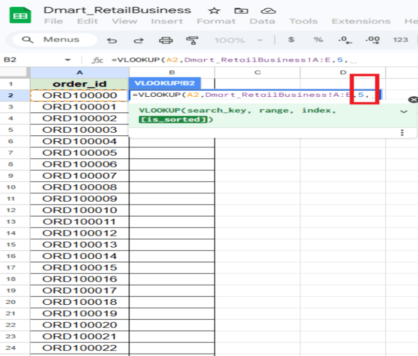
Using VLOOKUP, retrieve the sales value for a given order_id
1
Formula
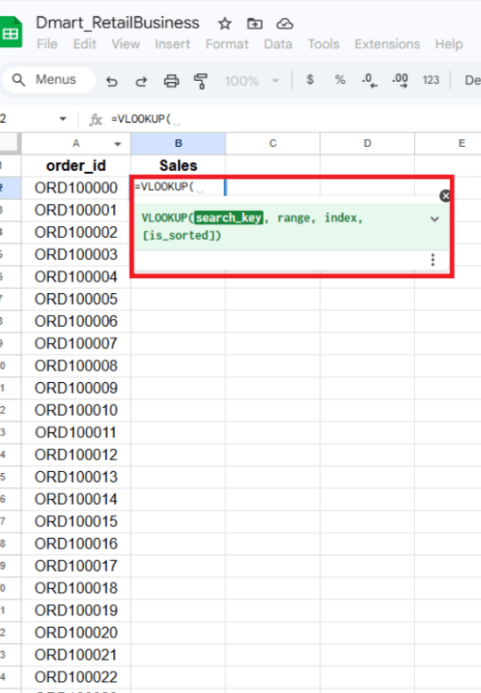
=VLOOKUP(search_key, range, index, [is_sorted])
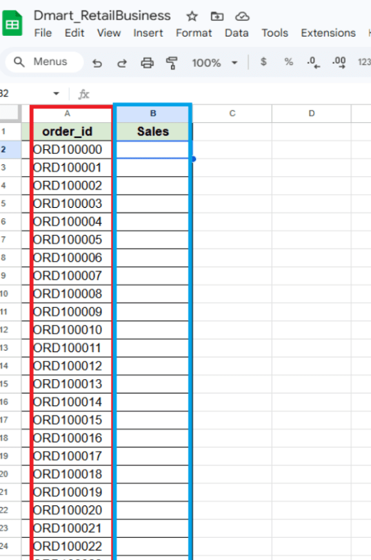
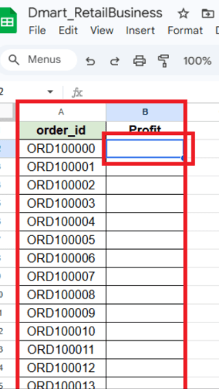
Create a new worksheet in the current workbook and copy all the order_id values from the first sheet into this new sheet.
a
VLOOKUP: VLOOKUP is an Excel function that searches for a value in the first column and returns a matching value from another column in the same row.
Click on an empty cell, type the equals sign (=), and enter the VLOOKUP function.
b
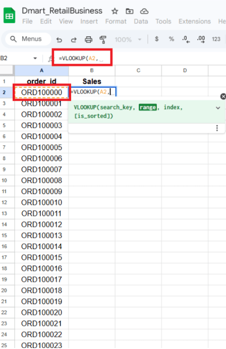
Select the lookup value (order_id), as this is the key used to search for the corresponding sales value.
c
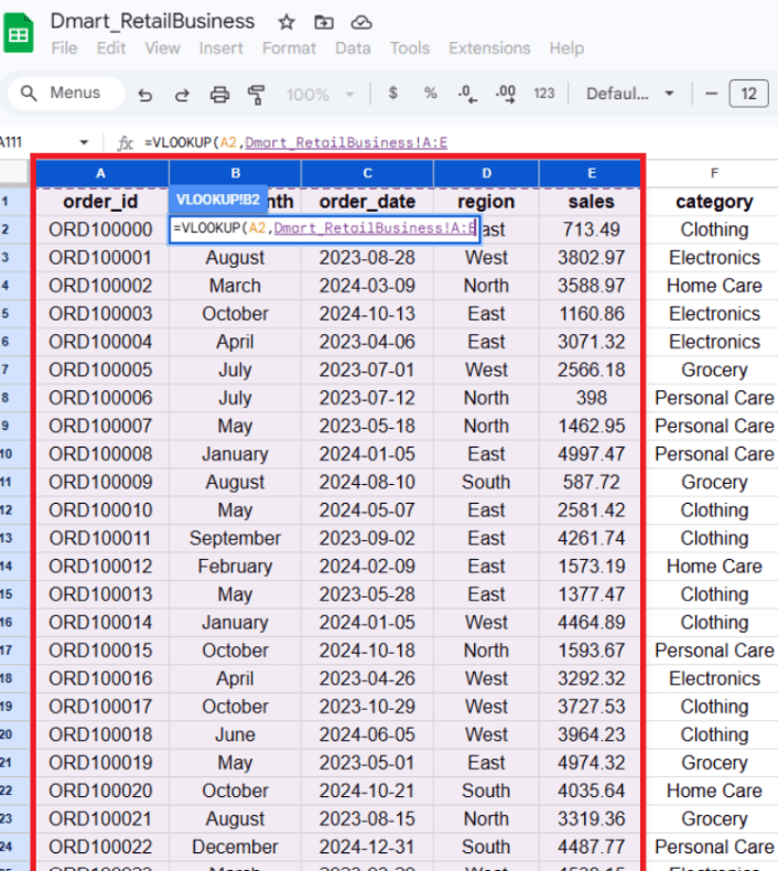
Select the table range that contains the data for the lookup.
d
Enter the column index number of the column that contains the sales value.
e
Enter the is_sorted =0
-tells Excel whether to return an approximate match (sorted data) or an exact match.
f
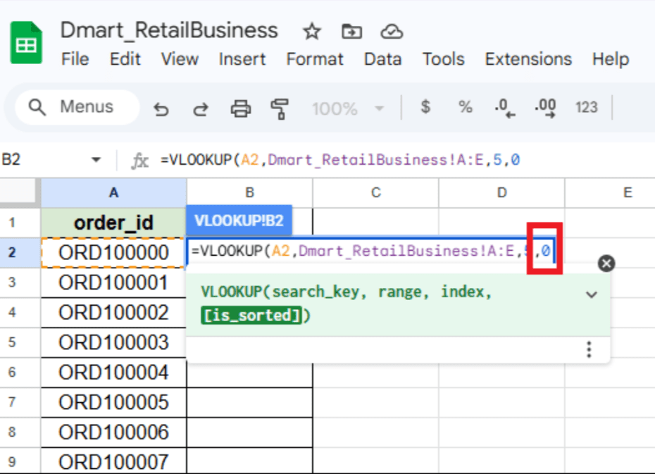
Press Enter to display the sales value for the selected order ID.
g
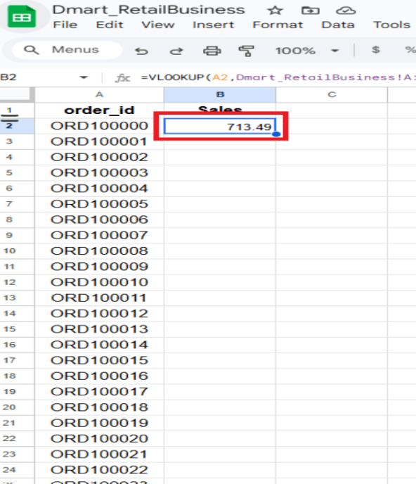
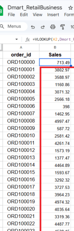
Double-click the bottom-right corner of the cell to drag the formula down and get sales values for all desired order IDs.
h
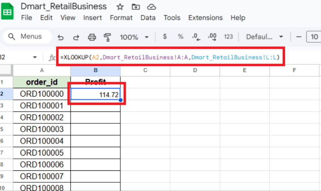
Retrieve the profit for a given order_id using XLOOKUP.
2
XLOOKUP: XLOOKUP finds a value in one column (or row) and returns a related value from another column (or row).
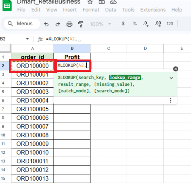
Click on an empty cell, type the equals sign (=), and enter the XLOOKUP function.
a
Formula
XLOOKUP(search_key, lookup_range, result_range, [missing_value], [match_mode], [search_mode])
Select the lookup value (order_id), as this is the key used to search for the corresponding Profit value.
b
Select the column (Order_ID) containing the data for the lookup.
c
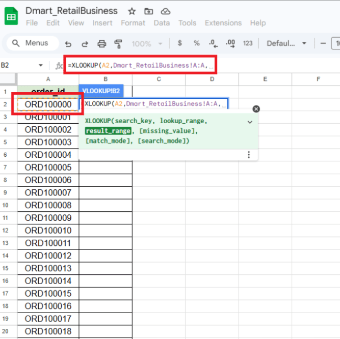
Enter the result_range(Profit).
d
Close the bracket and press Enter to display the profit value for the given order_ID.
e
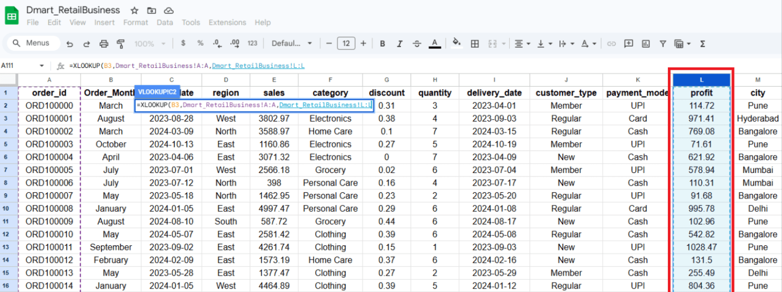
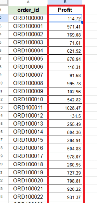
Double-click the bottom-right corner of the first profit cell to apply the formula and get profit values for all order IDs.
f
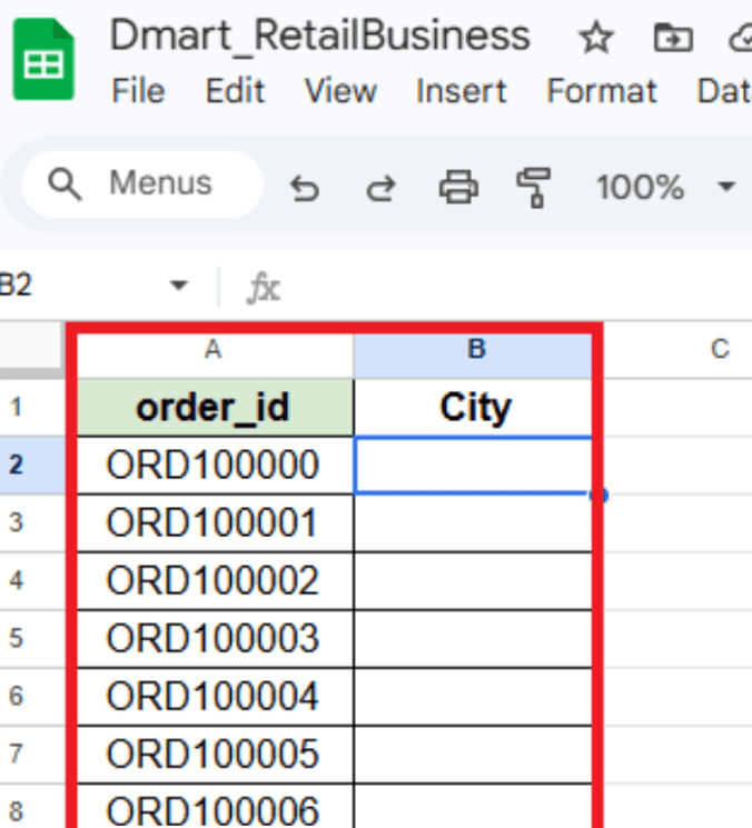
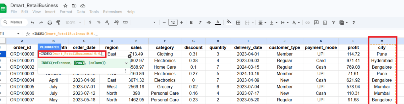
Retrieve the city where the order_id = ORD100020.
3
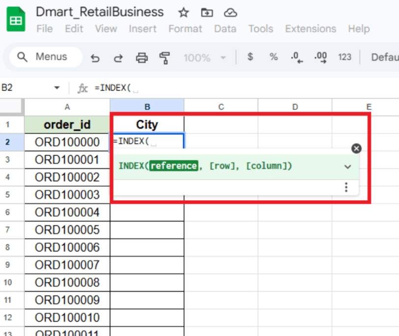
Formula
=INDEX(return_range, MATCH(lookup_value, lookup_range, 0))
Screenshots
Click on the empty cell in the city column.
a
INDEX-MATCH finds a value and returns related data from any position in the table.
Type (=) sign and index function.
b
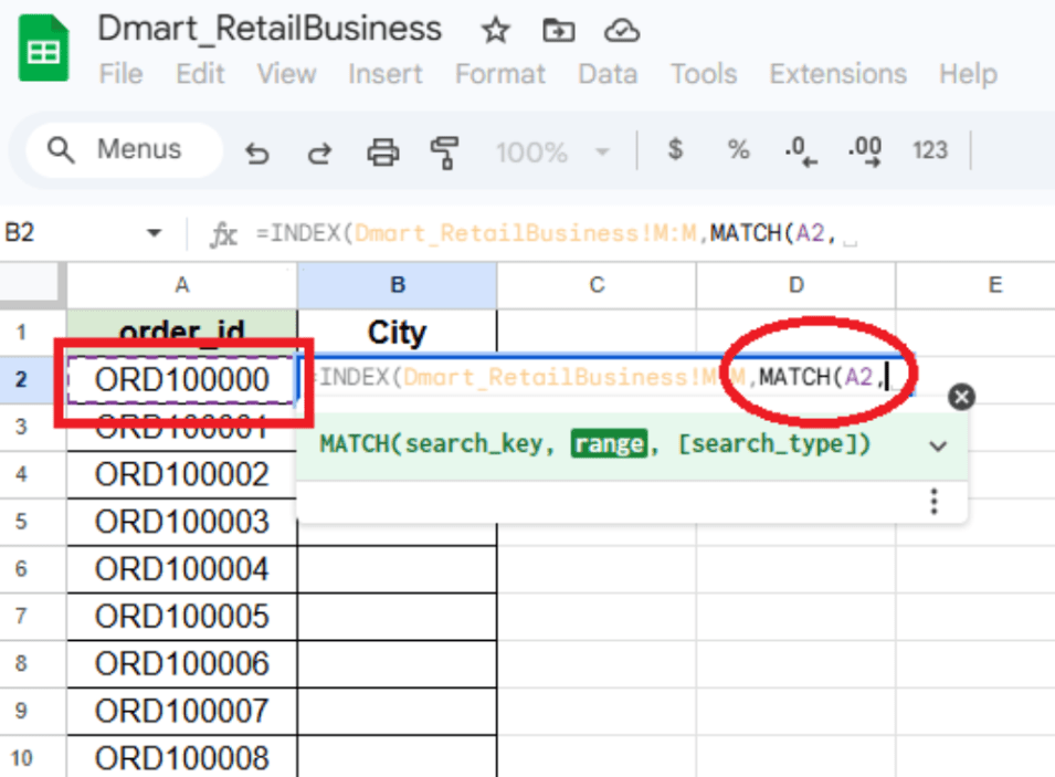
Type (=) sign and index function.
c
Type the MATCH function and select the order_id as the lookup value.
d
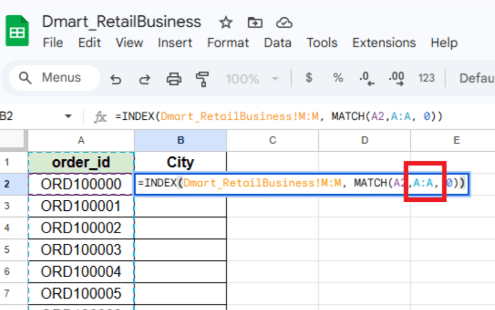
Select Order_id column as a search type.
e
Final output is seen here.
f
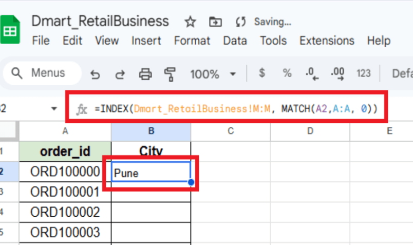
Double-click the bottom-right corner of the first city cell to apply the formula and get all values for all order IDs.
f
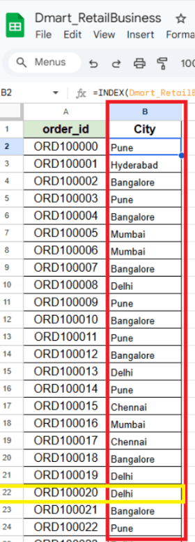
City name where the order_id = ORD100020 is Delhi is seen in above screenshot.
Task 2: Reports that can be filtered by region or product.
Select the Region column → go to the Insert tab → click on Slicer → choose the Region field → a slicer box will appear on the sheet → click on the specific region in the slicer → the data will be filtered to show only that region.
a
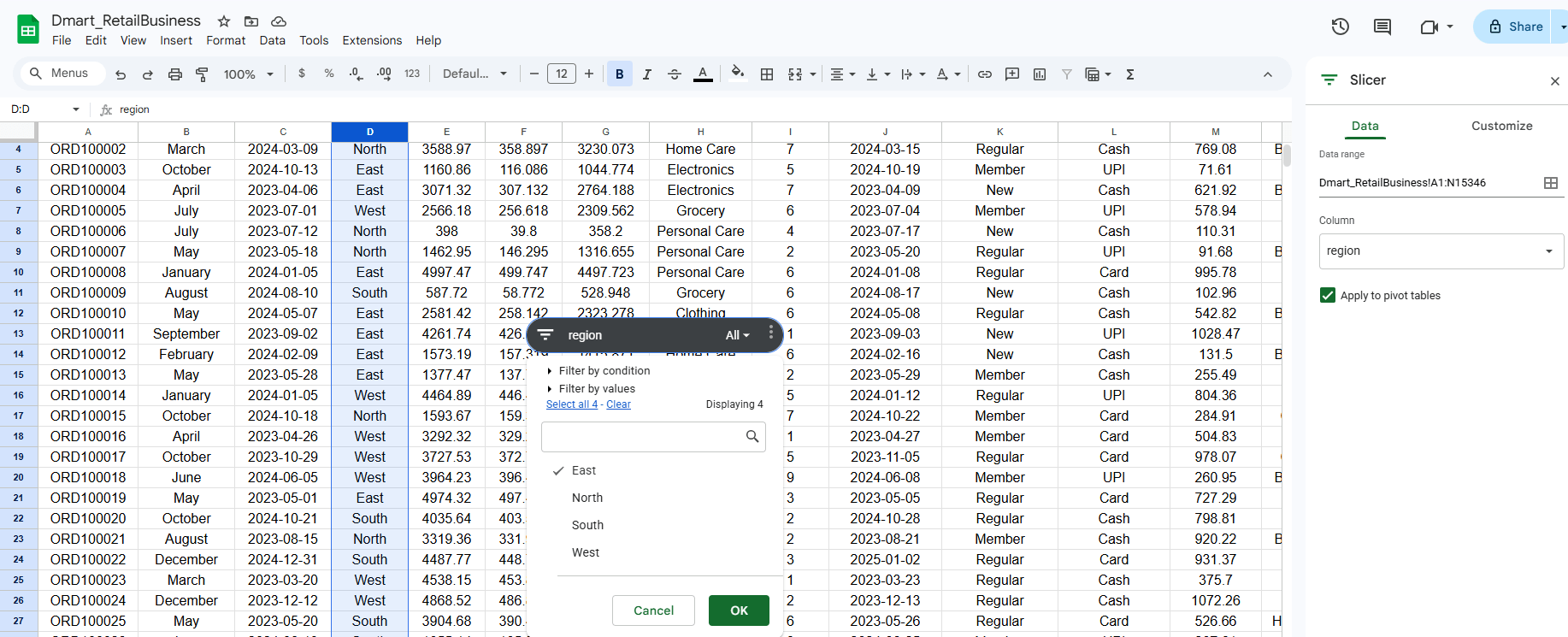
We will use a slicer, which allows users to interactively filter the data with just a click.
1
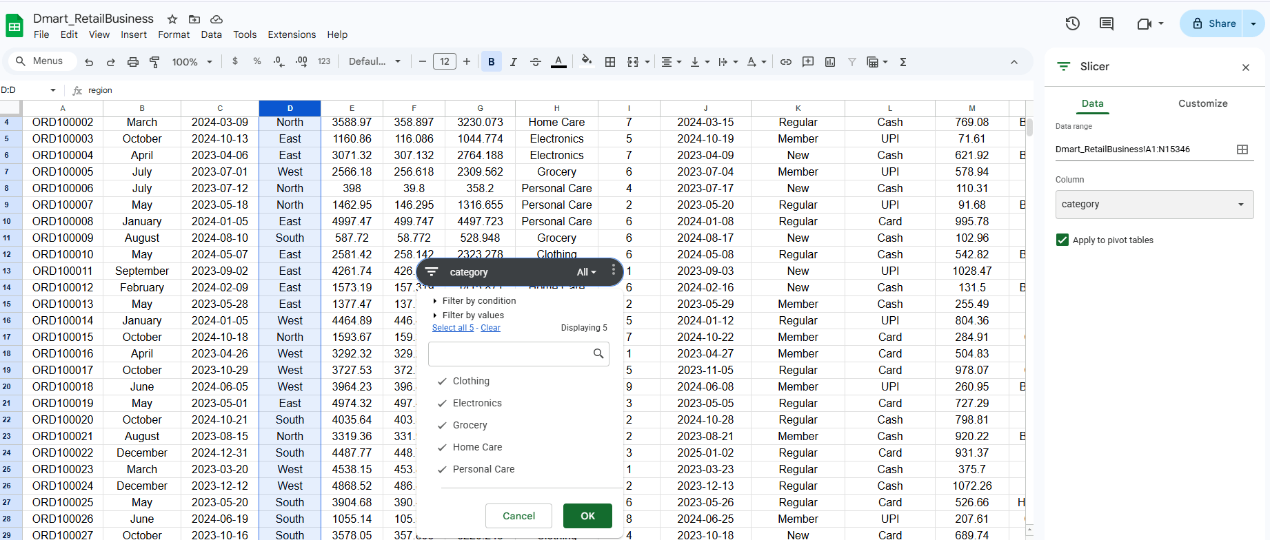
Select the Category column → go to the Insert tab → click on Slicer → choose the Category field → a slicer box will appear on the sheet → click on the specific category in the slicer → the data will be filtered to show only that category.
b
Great job!
You have successfully completed your lab Merging and Retrieving Data Using Lookup Functions.
In this lab, you have: Used lookup functions to retrieve data, Understood how to merge datasets, Applied slicers for interactivity, Created dynamic reports for creating Dashboard.
You are now ready to move to the next stage of data analysis.
Checkpoint
Git Push
git push origin branchNameTopic : PivotTable and Data Visualization Mastery
1) Creating PivotTables
2) Creating Graphs and Chart Types
3) Customizing Graphs and Sparklines
4) PivotCharts
Next-Lab Preparation