Competitive Equilibrium in the Edgeworth Box
Christopher Makler
Stanford University Department of Economics
Econ 51: Lecture 4
pollev.com/chrismakler

What song is playing right now?
Today's Agenda
- Trading in the Edgeworth Box at a common price ratio
- Net demand and net supply
- Solving for the equilibrium price ratio
- Alison and Bob example
- General Cobb-Douglas
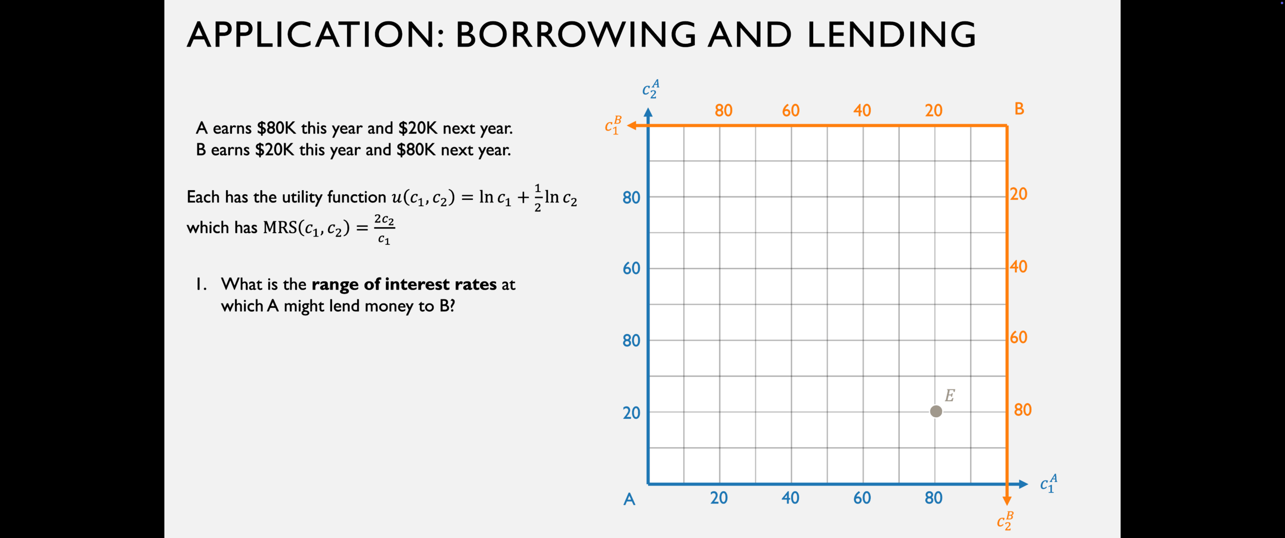
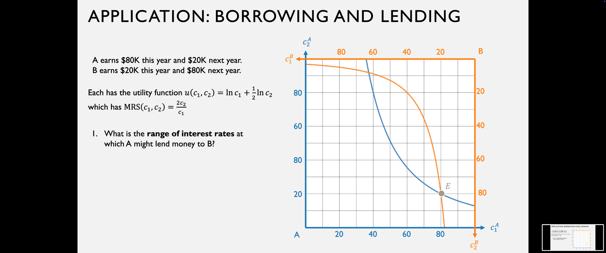
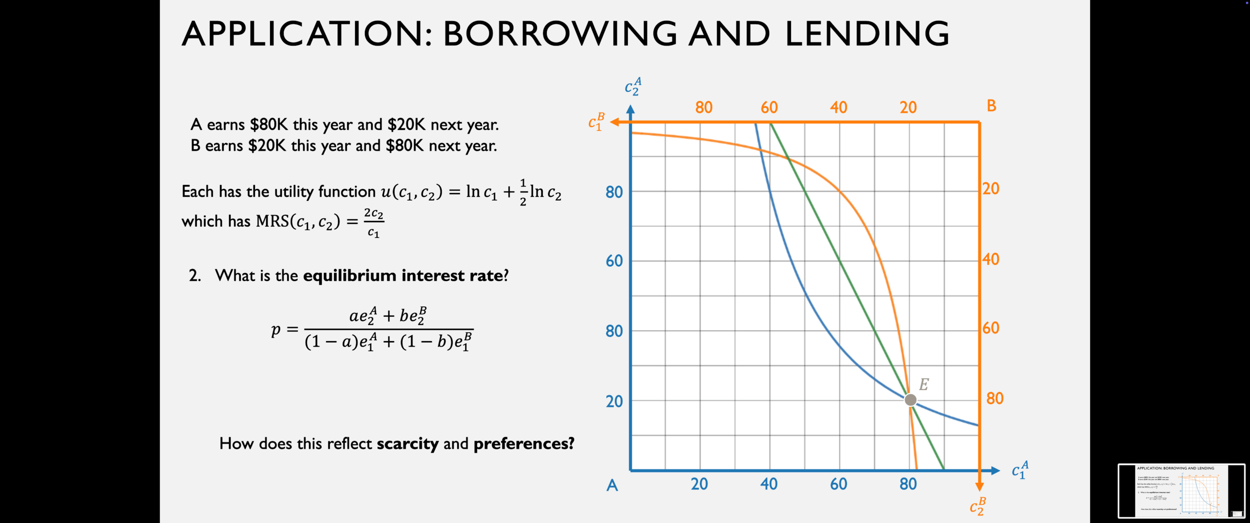
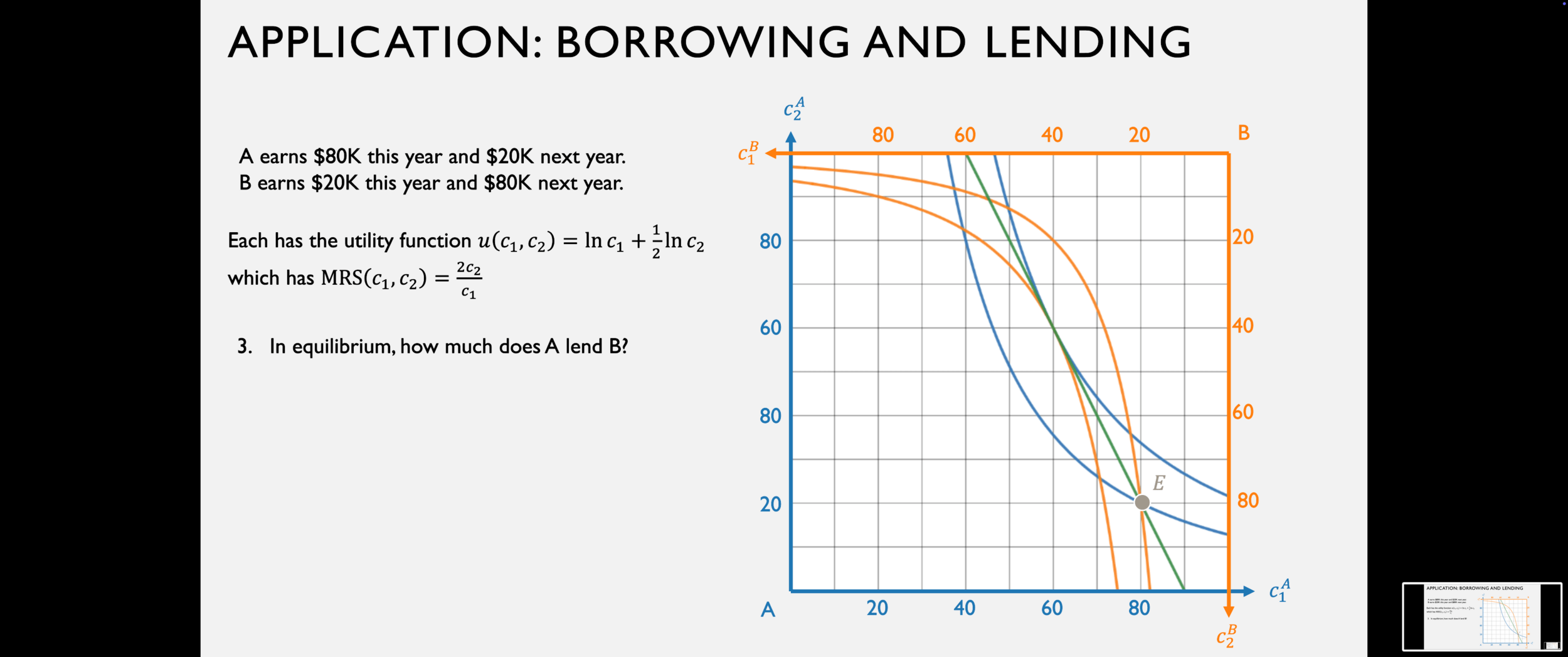
- Application to borrowing and lending
- First and second welfare theorems
From Last Time: Optimization from an Endowment
Bob has the Cobb-Douglas utility function \(u(x_1,x_2) = x_1x_2\) and an endowment of (8, 8)
Cobb-Douglas trick:
Since Bob has an endowment of (8,8), his "income" \(m\) is the value of that endowment
For this entire example, let's fix \(p_2 = 4\).
As we go through this example, work with a friend to solve it as well for Alison,
who has an endowment of (12,2).
The total quantity of a good
you want to consume (i.e. end up with)
at different prices.
Gross Demand
The transaction you want to engage in
(the amount you want to buy or sell)
at different prices.
Net Demand
Bob has the Cobb-Douglas utility function \(u(x_1,x_2) = x_1x_2\) and an endowment of (8, 8)
When is this positive?
So, Bob wants to buy good 1 when \(p_1 < 4\), and sell it when \(p_1 > 4\).
Remember that his utility function is \(u(x_1,x_2) = x_1x_2\), his endowment is (8,8), and \(p_2 = 4\).
MRS at endowment =
Price ratio =
Bob's MRS at his endowment is
Bob's net demand is
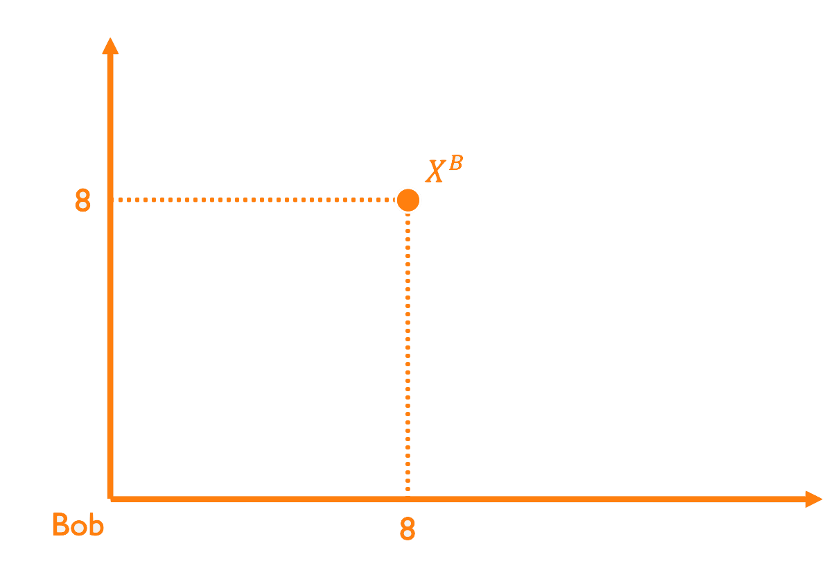
Bob
Endowment: (8,8)
Utility function: \(u(x_1,x_2) = x_1x_2\)
Bob's gross demand for good 1 is:
Bob
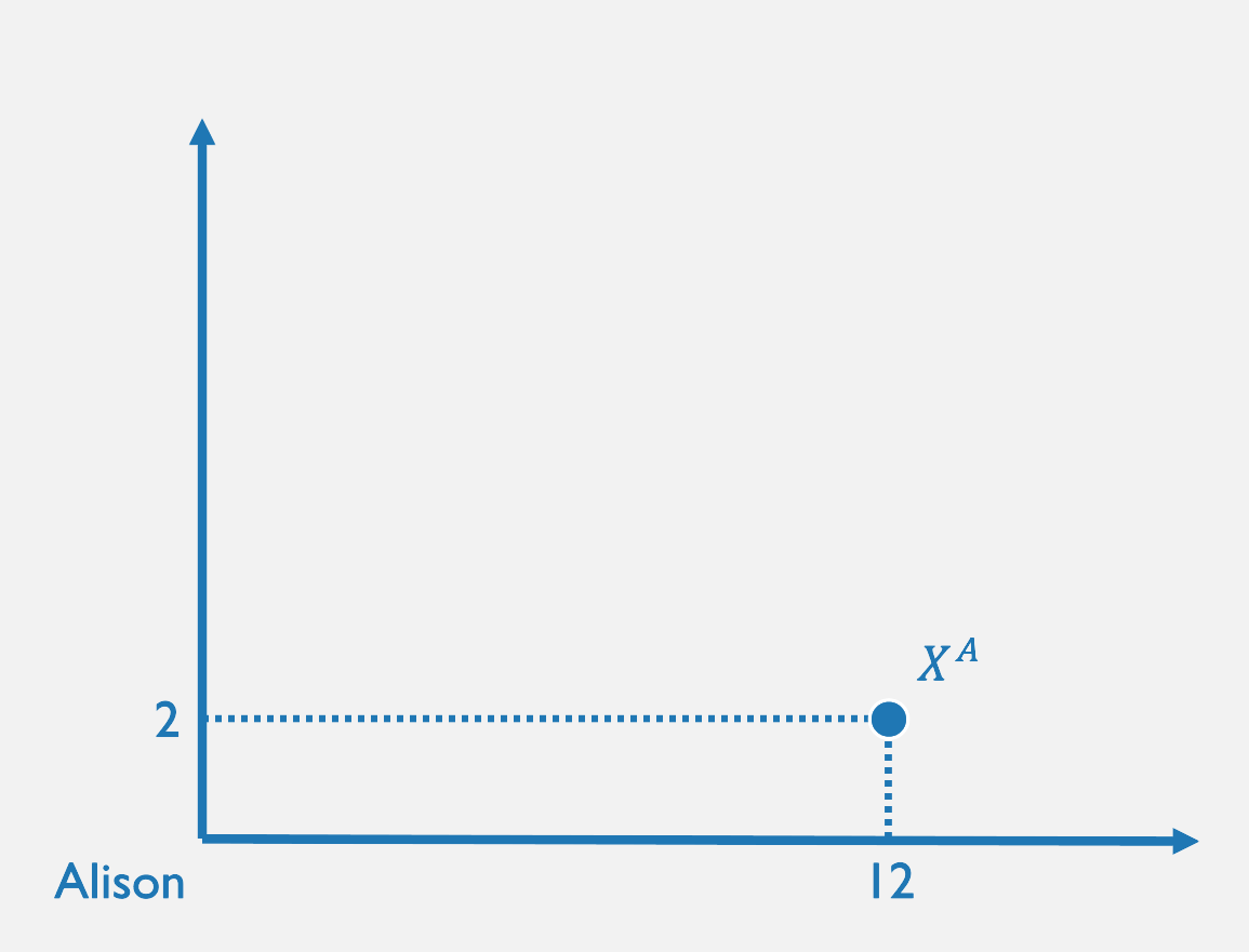
Endowment: (12, 2)
Utility function: \(u(x_1,x_2) = x_1x_2\)
Alison's gross demand for good 1 is:
Alison
Alison's MRS at her endowment is:
Alison's net demand is:
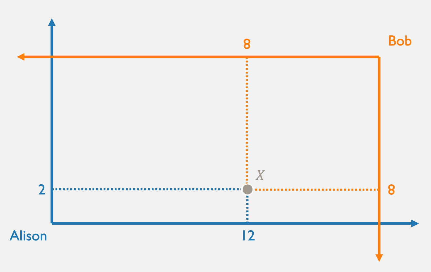
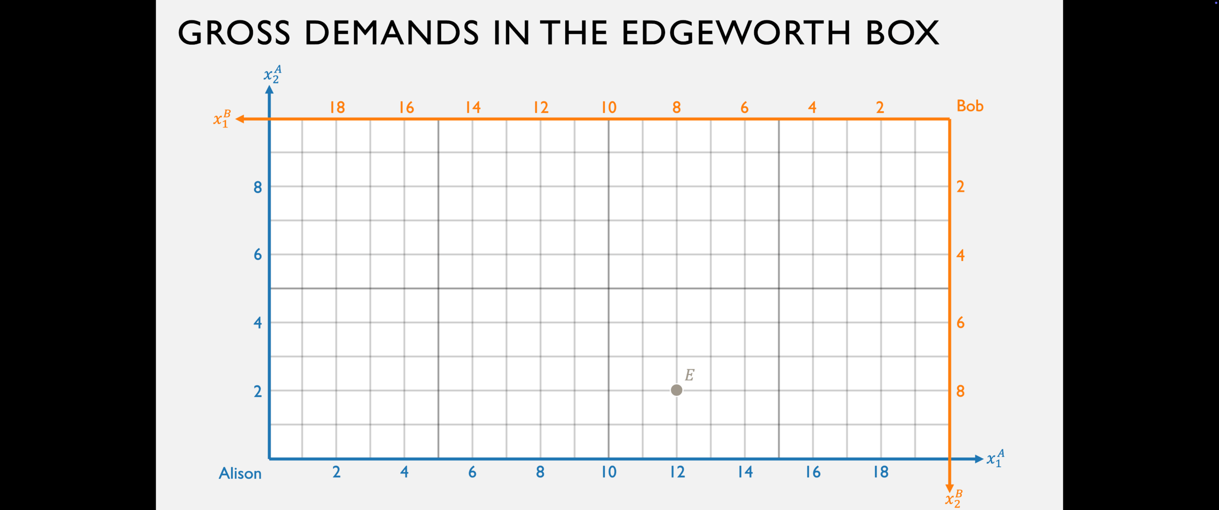
Back to the Edgeworth Box...

From Bundles to Allocations
From Bundles to Allocations
Trade in the Edgeworth Box
- Suppose both agents believe they can trade at some price ratio \(p_1/p_2\).
- Then they share a common budget line in the Edgeworth Box.
...but where do they want to trade to?
Preferences in the Edgeworth Box
What does the "lens" of overlap represent?
How is the existence of this lens related to
the agents' marginal rate of substitution (MRS) at point \(X\)?
Bob's MRS at his endowment is
Bob
Bob
Alison
Alison's MRS at her endowment is:
Alison wants to sell good 1 if:
Bob wants to buy good 1 if:
Between these two price ratios, Alison wants to sell good 1 and Bob wants to buy good 1.
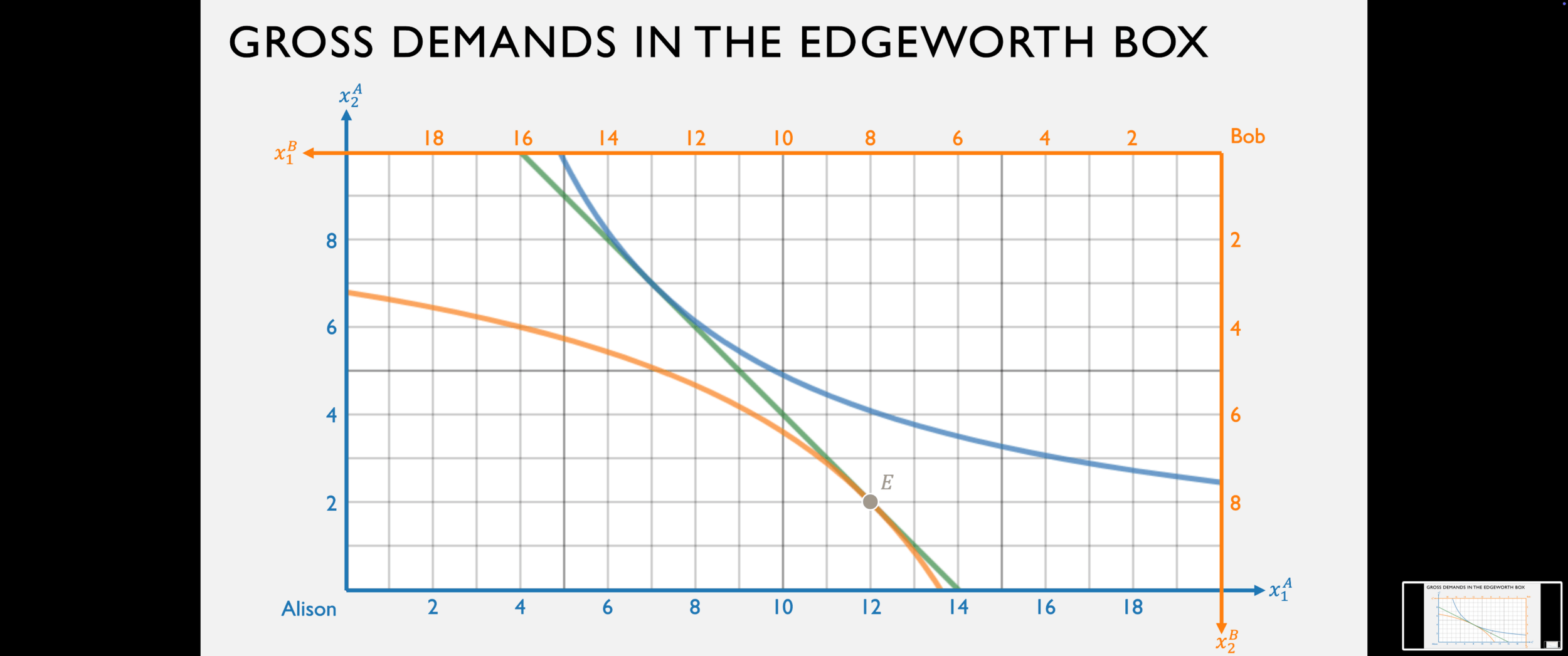
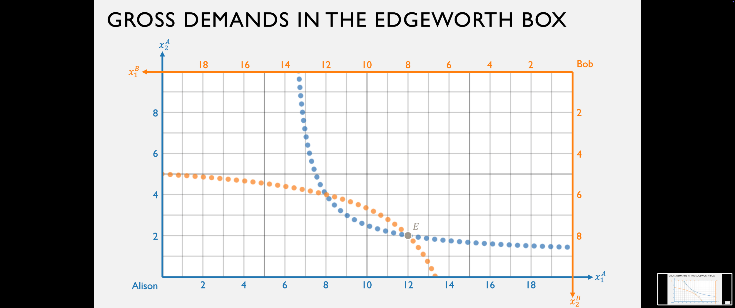
Bob's gross demand for good 1 is:
Bob
Alison's gross demand for good 1 is:
Alison
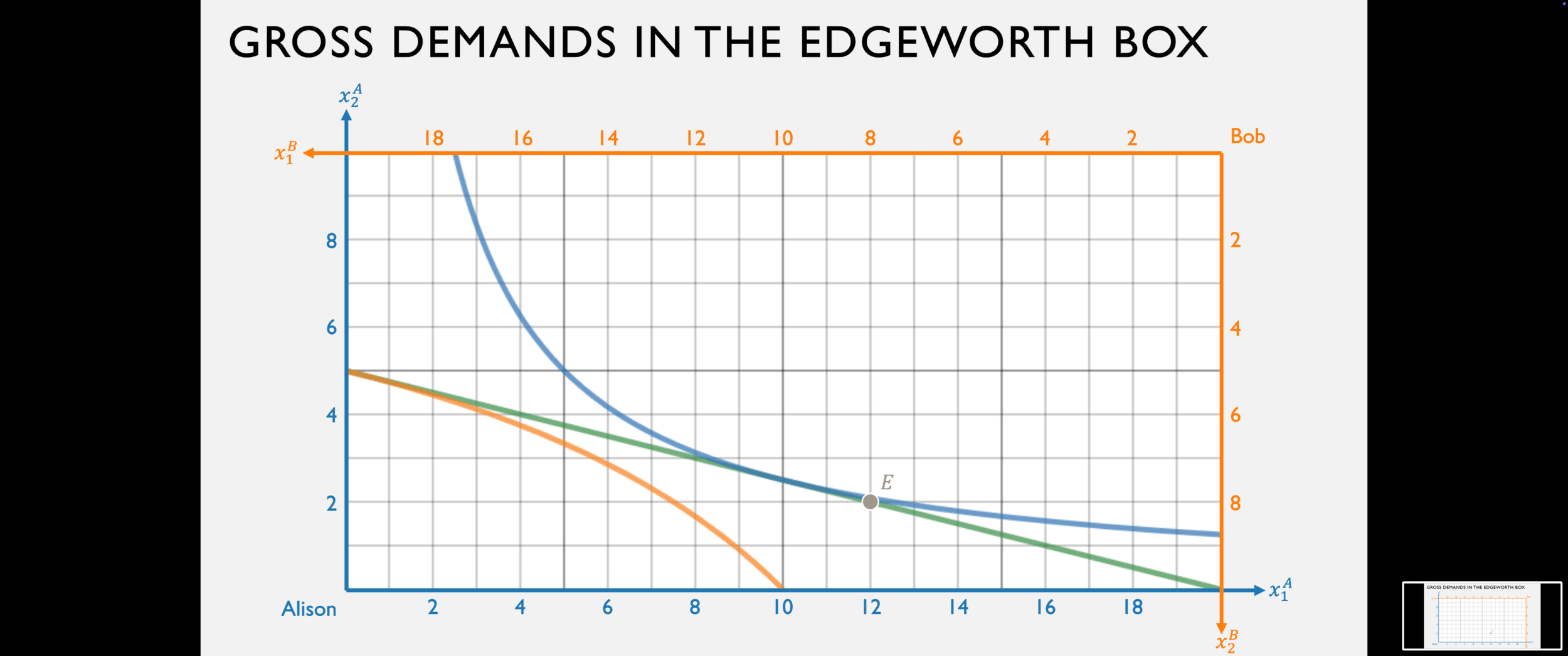

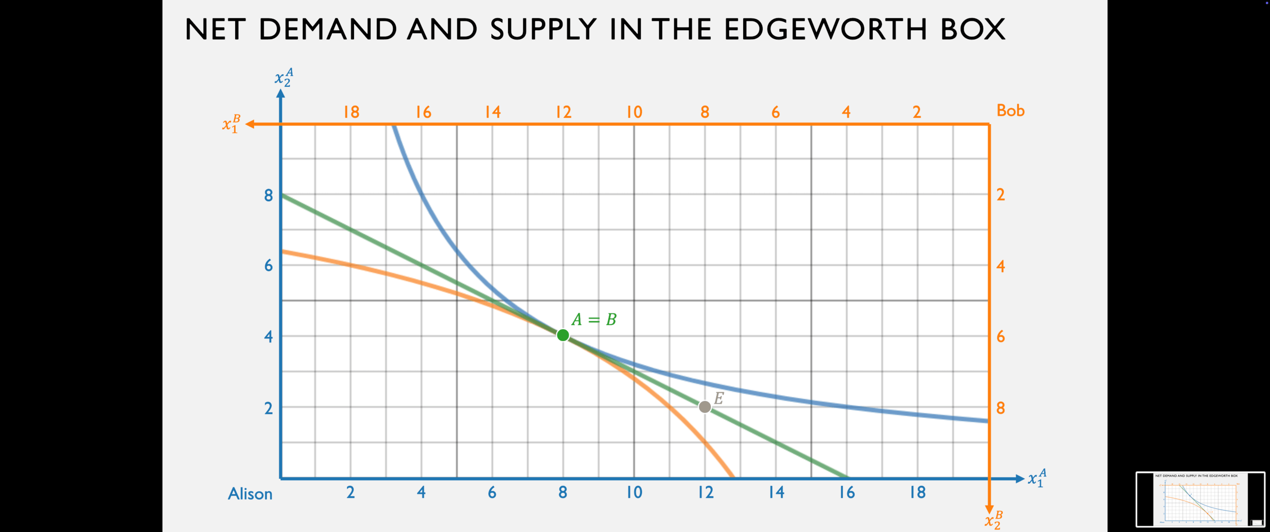
Net Demand and Supply
- The gross demands tell us where each agents wants to trade to at any given price ratio.
- We can think about this same data in terms of net demand and net supply.
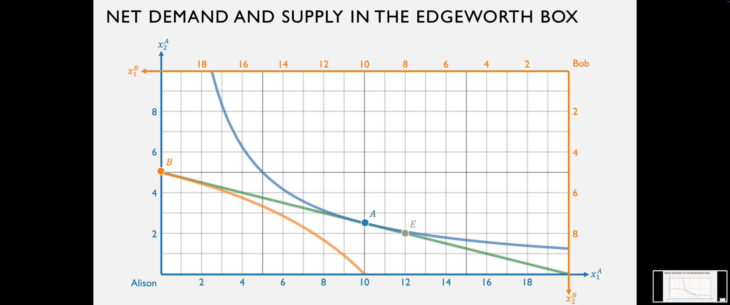
Bob's gross demand for good 1 is:
Alison's gross demand for good 1 is:
His net demand for good 1 is:
Her net supply of good 1 is:
Bob demands 12
Alison supplies 2
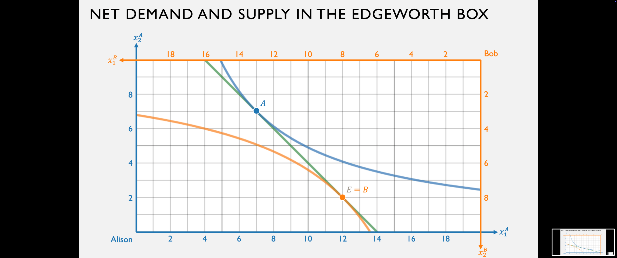
Bob's gross demand for good 1 is:
Alison's gross demand for good 1 is:
His net demand for good 1 is:
Her net supply of good 1 is:
Bob demands 4
Alison supplies 4
Bob's gross demand for good 1 is:
Alison's gross demand for good 1 is:
His net demand for good 1 is:
Her net supply of good 1 is:
(Bob demands 0)
Alison supplies 5
Bob's net demand for good 1 is:
Alison's net supply of good 1 is:
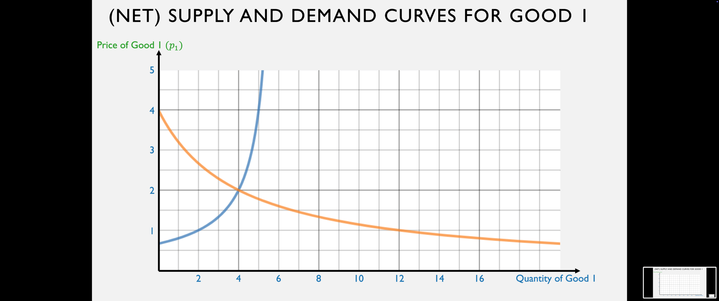
Solving for Equilibrium
Bob's net demand for good 1 is:
Alison's net supply of good 1 is:
Just like we always do, set these equal to one another and solve for the equilibrium price!
Bob's net demand for good 1 is:
Alison's net supply of good 1 is:
Just like we always do, set these equal to one another and solve for the equilibrium price!
Solving for general Cobb-Douglas utility functions
The parameter \(a\) measures how much A likes good 1,
and the parameter \(b\) measures how much B likes good 1.
Solving for general Cobb-Douglas utility functions
The parameter \(a\) measures how much A likes good 1,
and the parameter \(b\) measures how much B likes good 1.
Formula for the equilibrium price ratio:
In our example with Alison and Bob, we had: \(a = {1 \over 2}, e_1^A = 12, e_2^A = 2; b = {1 \over 2}, e_1^B = 8, e_2^B = 8\):
In this example, both Alison and Bob liked the two goods equally. Why wasn't the price ratio 1?
Solving for general Cobb-Douglas utility functions
The parameter \(a\) measures how much A likes good 1,
and the parameter \(b\) measures how much B likes good 1.
Formula for the equilibrium price ratio:
What happens to the relative price of good 1
if people like good 1 more (that is, \(a\) and \(b\) are higher)?
What happens to the relative price of good 1
if there is more good 1 in the world (that is, \(e_1^A\) and \(e_1^B\) are higher)?
In competitive equilibrium in an exchange economy,
the price ratio reflects two fundamental things:
the preferences of the agents, and
the relative scarcity of the goods.


Fundamental Theorems of Welfare Economics
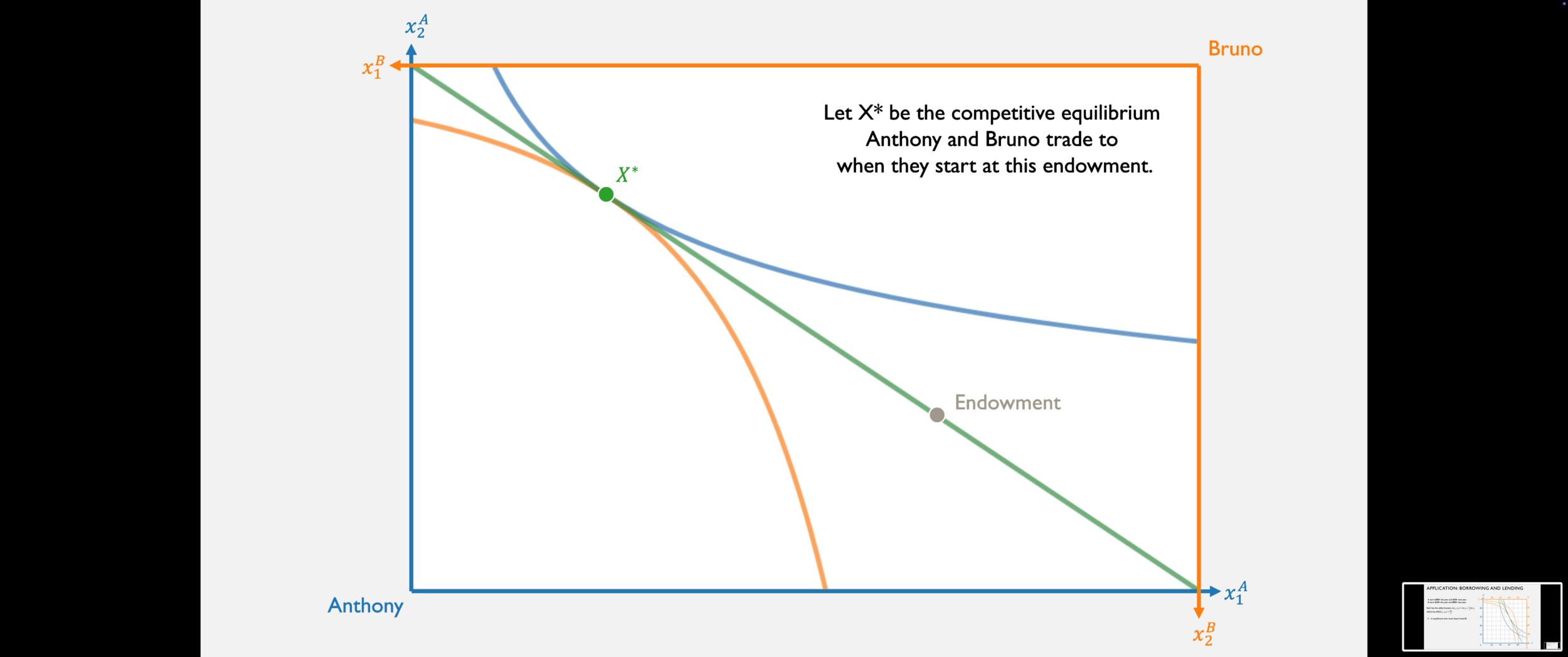
- First Welfare Theorem: If an allocation \(X^*\) is a competitive equilibrium, then it is Pareto efficient.
- Second Welfare Theorem: When preferences are convex, any Pareto efficient allocation is an equilibrium for some set of prices and some endowment.
The First Welfare Theorem
- Formally: If an allocation \(X^*\) is a competitive equilibrium, then it is Pareto efficient.
- Intuitively: Markets are efficient. If you just let everyone do what's best for themselves, you end up with a Pareto efficient outcome. Libertarianism FTW!
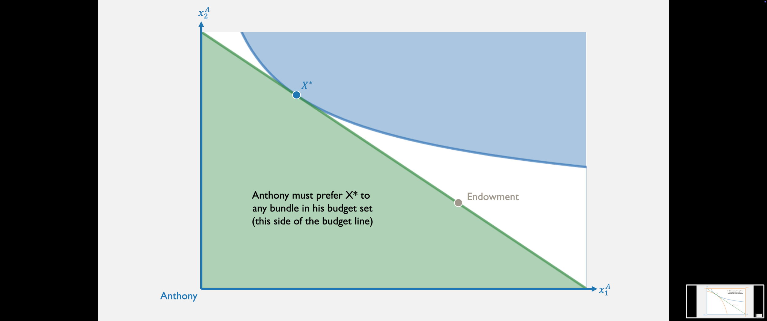
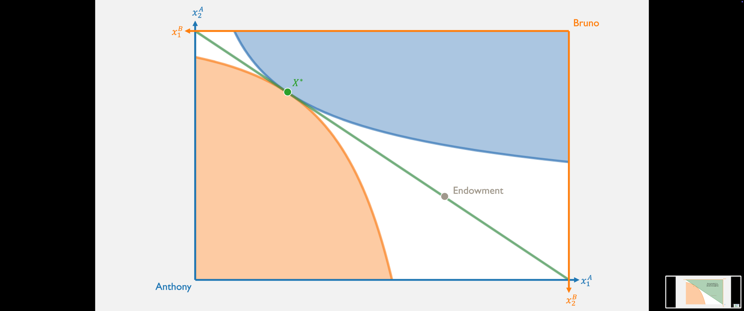
Since Anthony's preferred set is entirely on this set of the budget line...
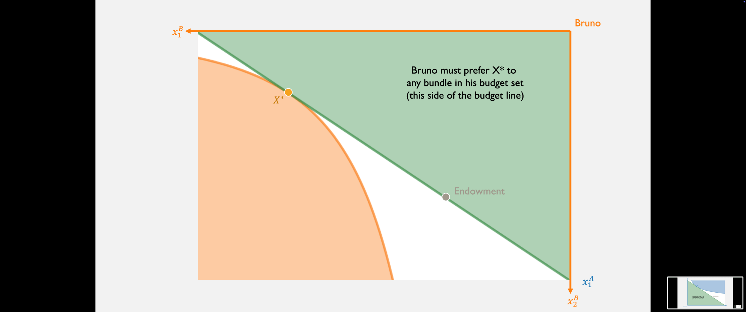
...and Bruno's preferred set is entirely on this side of the budget line...
...then X* must be Pareto efficient!
Second Welfare Theorem
- Under certain assumptions on preferences, every Pareto efficient allocation can be achieved as a competitive market equilibrium for some initial set of endowments.
- This sounds a lot like communism...
- ...but what if we think about establishing "endowments" in a more philosophical way?
Application: Smoking
Two roommates, Ken and Chris.
Ken is a smoker who can smoke up to 10 hours per day.
Chris is a non-smoker and dislikes Ken's smoking.
Preferences
Each have preferences over how much Ken smokes (good 1) and money (good 2).
Preferences
Each have preferences over how much Ken smokes (good 1) and money (good 2).
Suppose we define property rights over smoking.
This is like an endowment:
Let's assume Chris and Ken each start with $100.
Equilibrium
If we allow them to trade from their endowment, they'll end up on the contract curve — at an efficient allocation!
Next Time
- Where does the Edgeworth box come from?
- Where do the initial "endowments" come from?
- We'll step back and look at production decisions...