Financial Instruments:
Bonds and Futures
Christopher Makler
Stanford University Department of Economics
Econ 50: Lecture 13
Warm-Up Exercise: Expected Value
If a random variable \(X\) takes on values \(x_1,x_2,x_3,...,x_n\) with probabilities \(\pi_1,\pi_2,\pi_3,...,\pi_n\), where the \(\pi\)'s all add up to 1, then the expected value of \(X\) is
Example:
Suppose there is a 50% chance it will rain tomorrow,
If it rains, there is an 80% chance it will rain 10mm,
and a 20% chance it will rain 20mm.
What is the expected value of the amount of rain?
pollev.com/chrismakler

Applications of Uncertainty and Intertemporal Choice
Futures
Buying money in states of the world
Prediction Markets
Problems of insider trading and market manipulation
Bonds
Duration
Inflation
Risk of Default
Futures and Prediction Markets
Risk Aversion
You prefer having E[c] for sure to taking the gamble
You're indifferent between the two
You prefer taking the gamble to having E[c] for sure
Marginal Rate of Substitution
Where do the values of \(c_1\) and \(c_2\) come from?
- Up to now, we've been talking about your preferences over lotteries.
- What if you could buy a lottery in the same way as you could buy a bundle of goods?


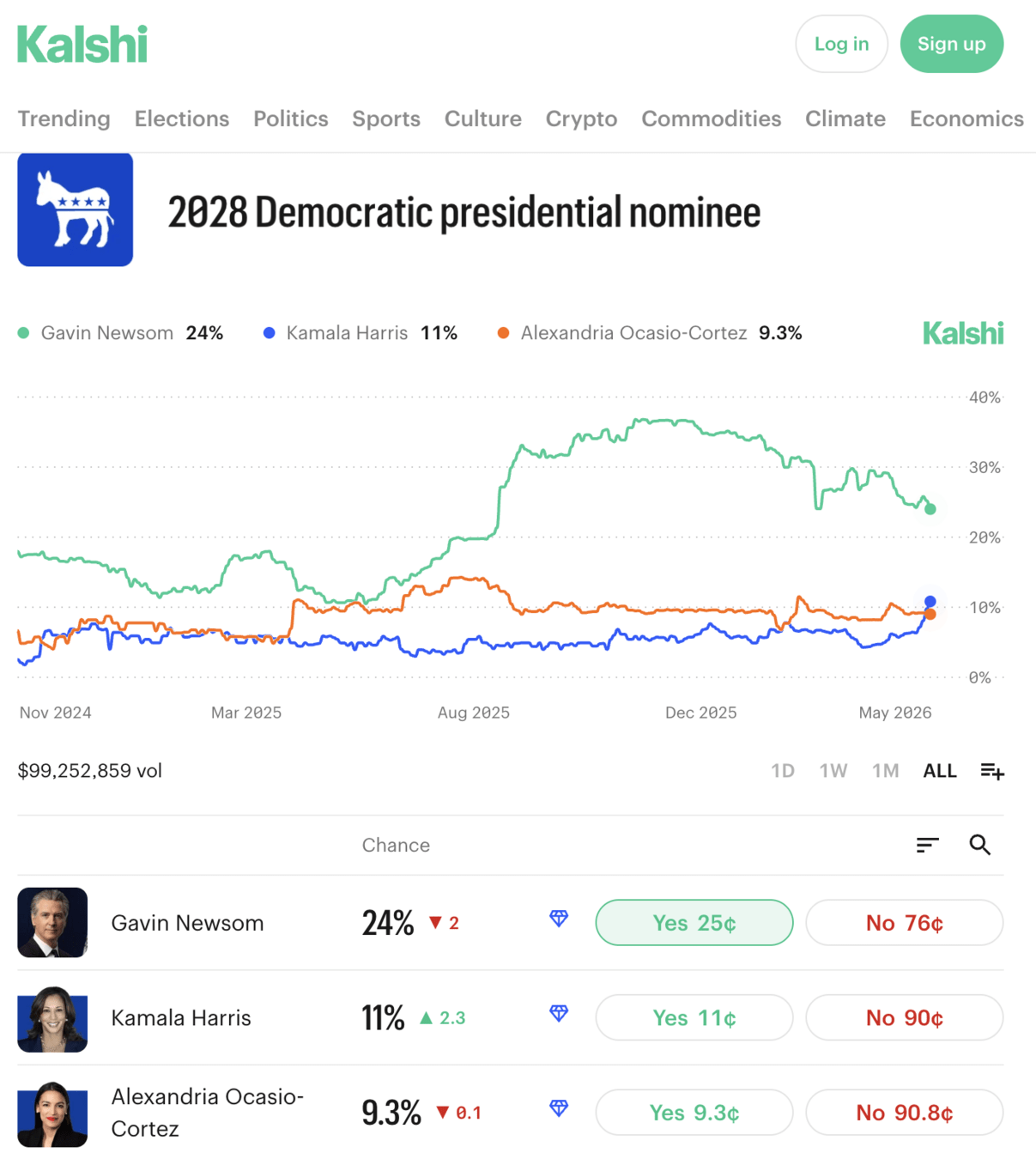
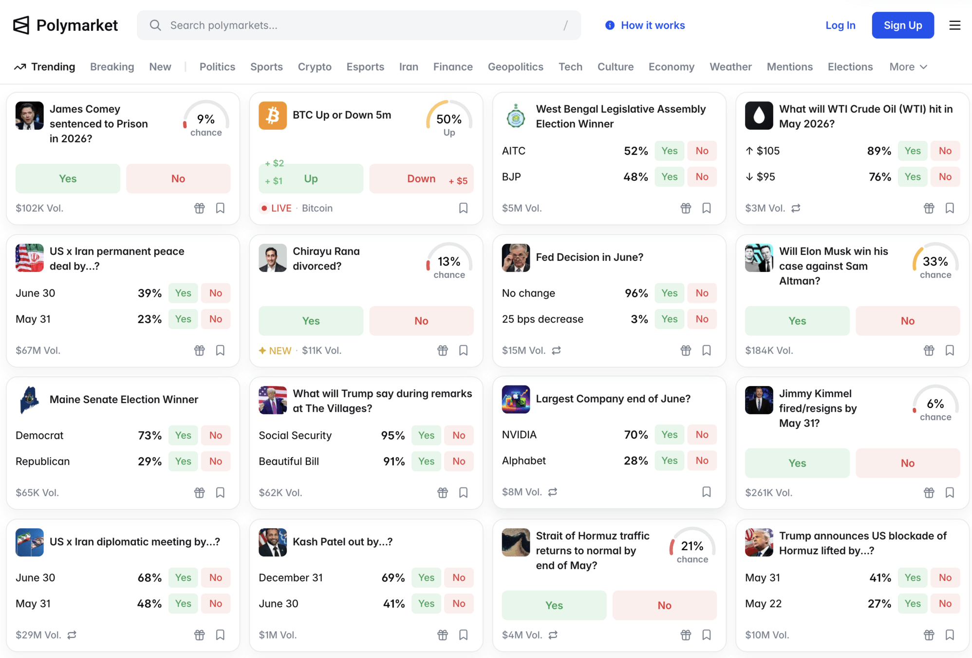
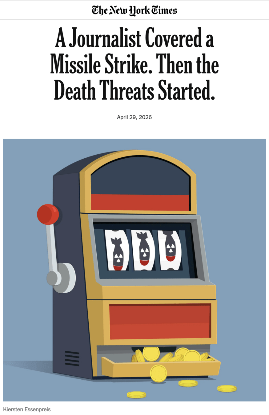
Prediction markets like Kalshi and Polymarket let you buy a contract that pays $1 if an event occurs.
You can either buy a contract saying the event will occur, or that it will not occur. These must add up to 1, with possible rounding errors.
So, if \(c_1\) is your consumption if the event occurs, and \(c_2\) is your consumption if it doesn't occur, these prices are \(p_1\) and \(p_2\)!
Your value function for money in any state of the world is \(v(c) = c^r\).
Suppose you have $300 in your pocket, and you believe Gavin Newsom will win with some probability \(\pi > 0.25\).
You can buy money in state of the world 1 for \(p_1 = 0.25\). How much should you buy?
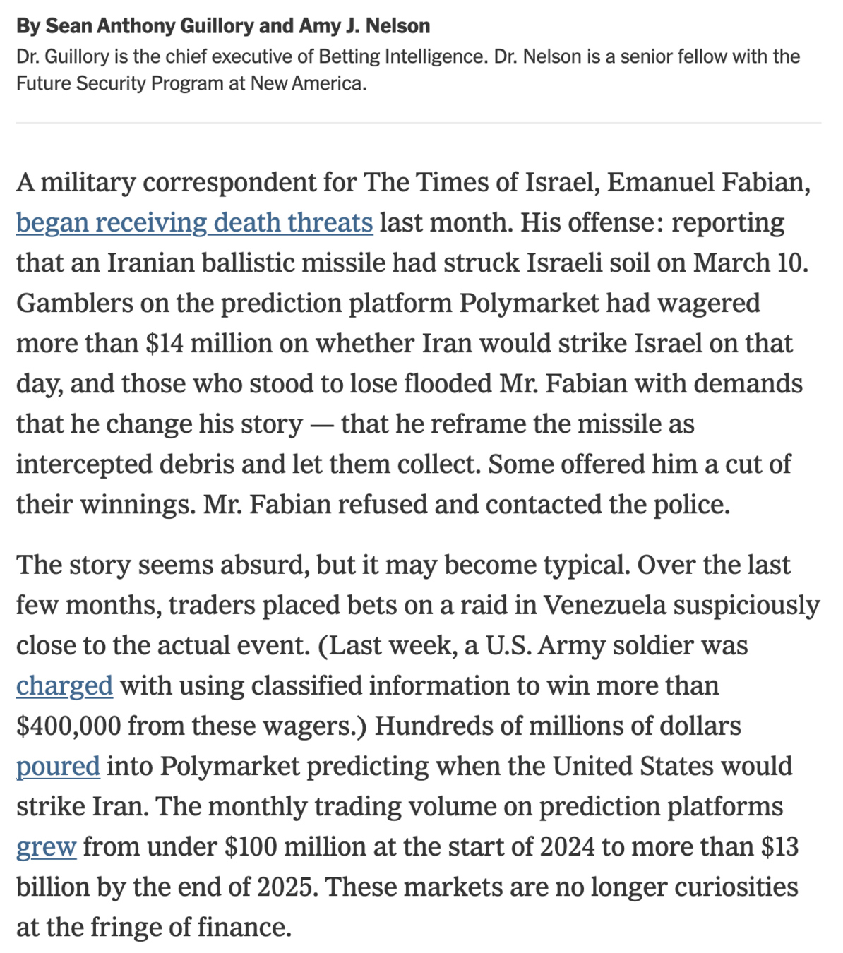
Prediction Markets: The Good, the Bad, and the Ugly
- Good: Information has economic value, and prediction markets can provide real-time data on the "wisdom of crowds."
- Bad: insider trading - traders know whether an event will happen
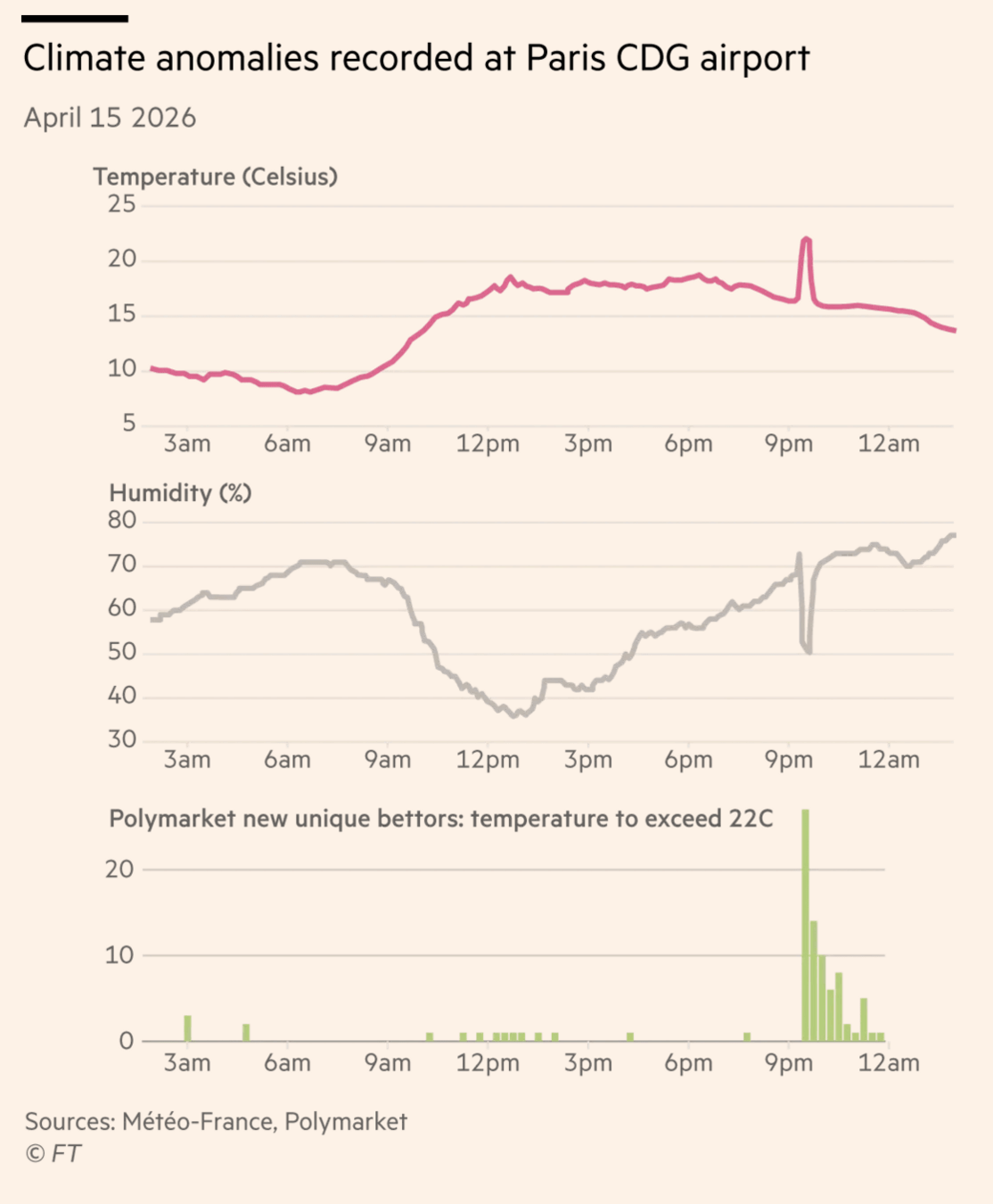
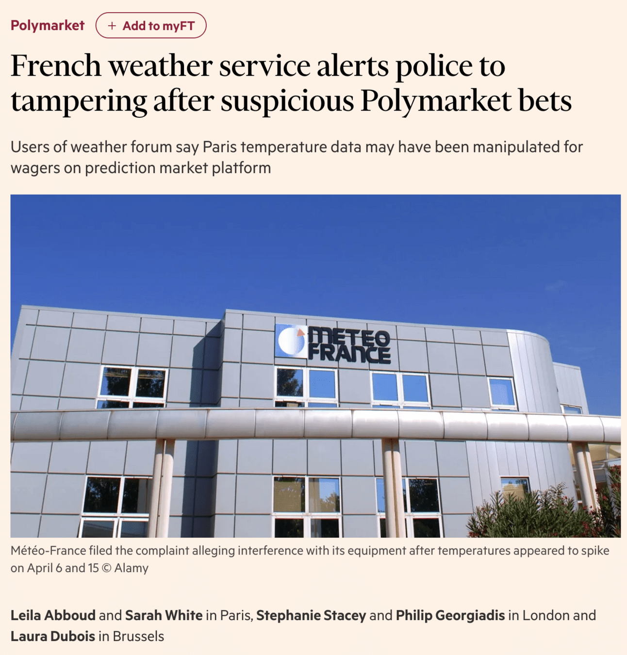
- Ugly: Risk of market manipulation - traders can influence the odds of an event happening
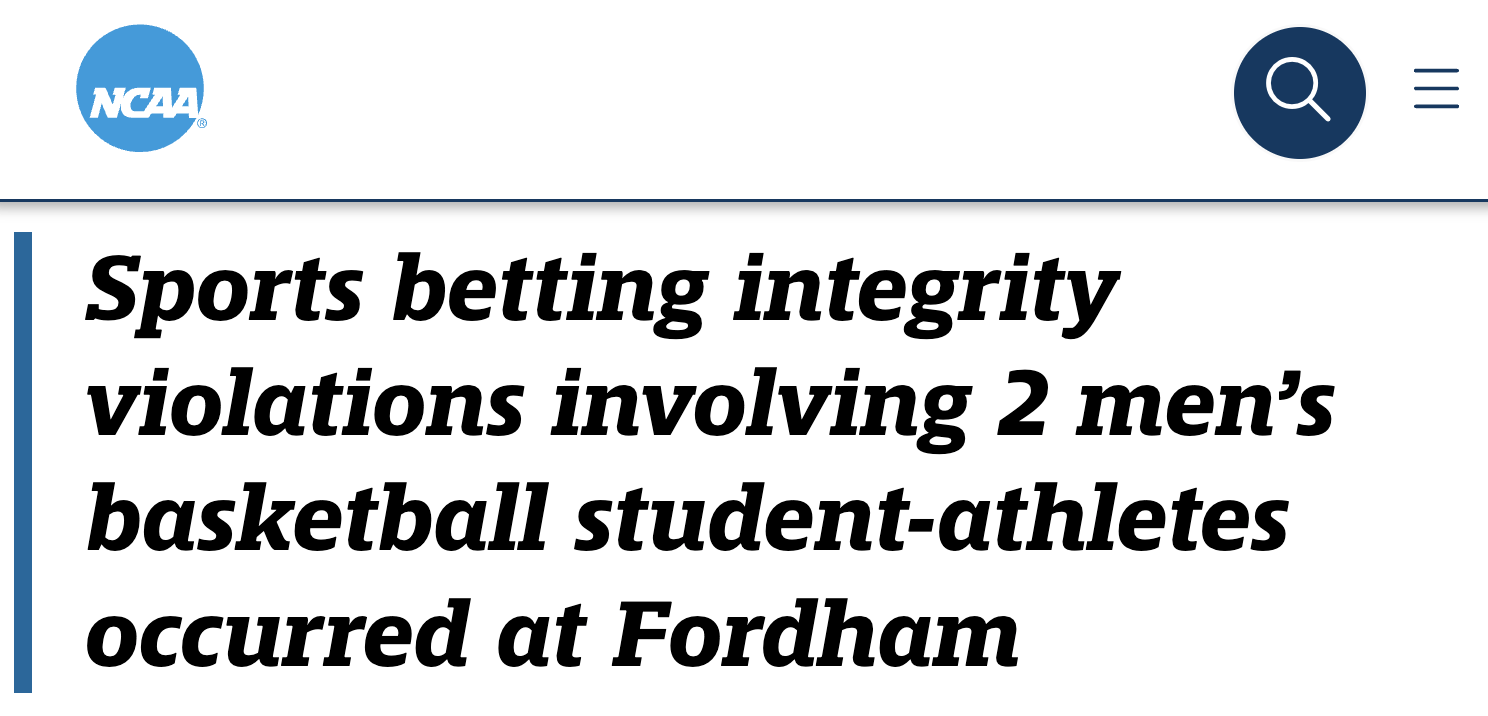
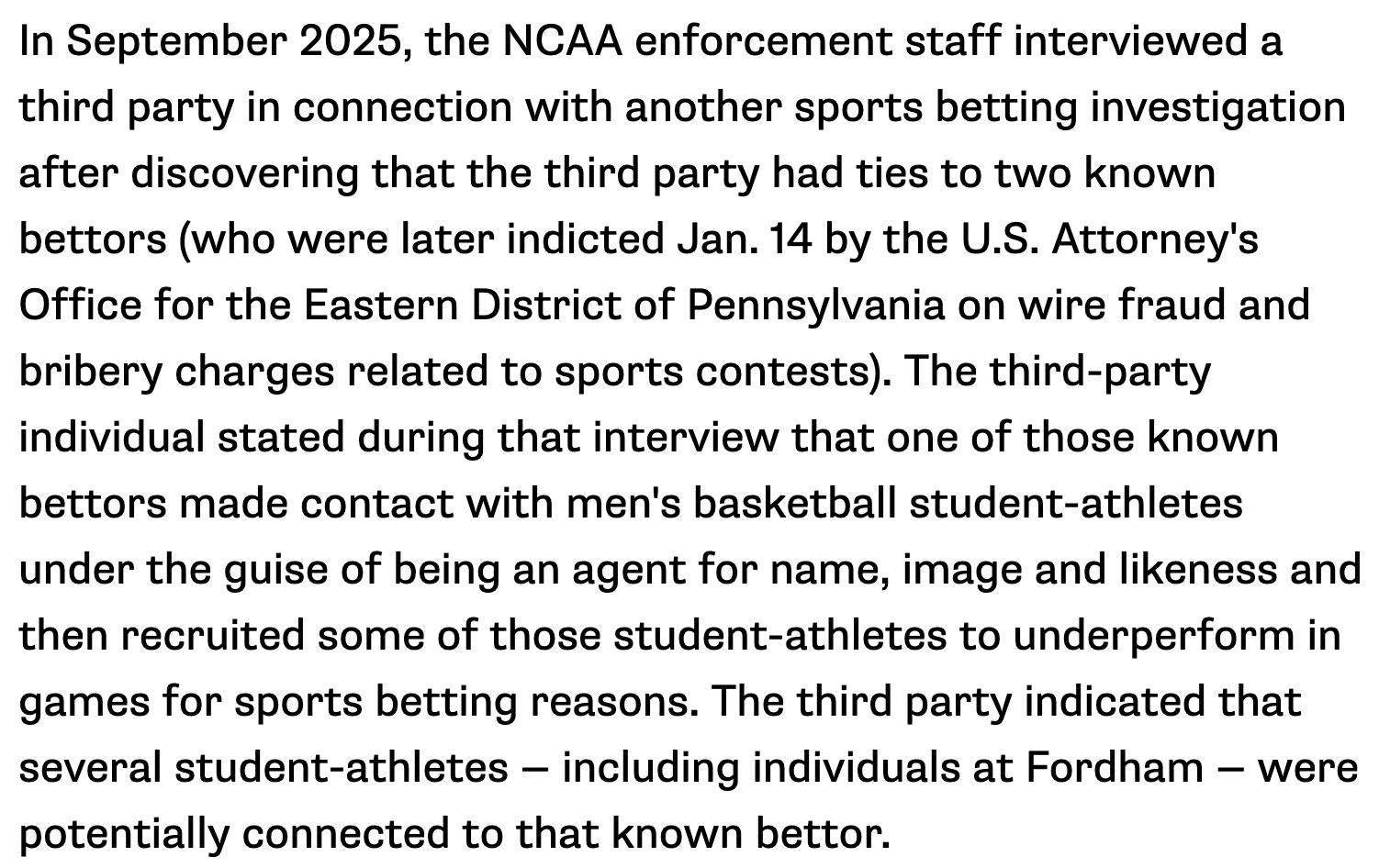
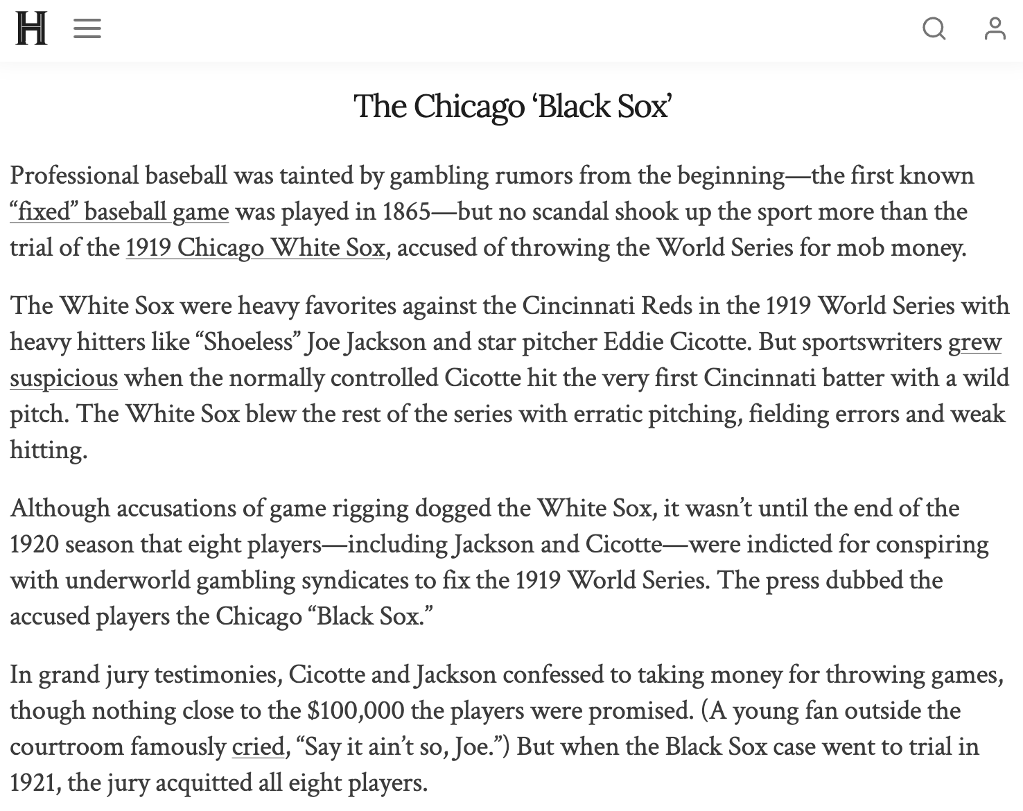
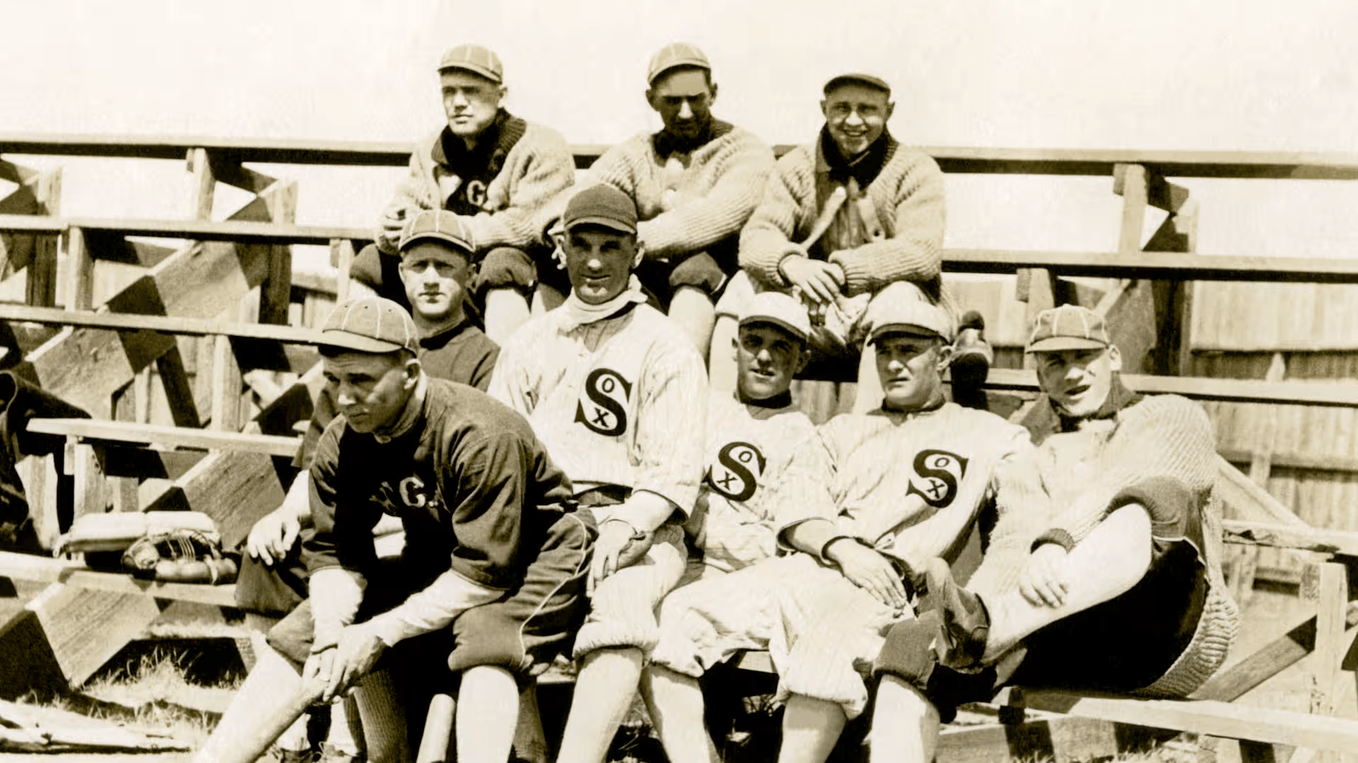
Lest you think this is a new phenomenon...
An important note
Prediction markets walk a fine line between investing, risk hedging, and gambling.
Markets for risky assets are a core subject of econ; but gambling addiction is a serious problem.
If you or someone you love has a problem with gambling, there is help. Reach out.
Bonds
Inflation and Real Interest Rates
Suppose there is inflation,
so that each dollar saved can only buy
\(1/(1 + \pi)\) of what it originally could:
Up to now, we've been just looking at
dollar amounts in both periods
We call \(r\) the "nominal interest rate" and \(\rho\) the "real interest rate"
For low values of \(r\) and \(\pi\), \(\rho \approx r - \pi\)
"Present Value" for two periods
Beyond Two Periods
If you save \(s\) now, you get \(x = s(1 + r)\) next period.
The amount you have to save in order to get \(x\) one period in the future is
Remember how we got this...
If you save \(s\) now, you get \(x = s(1 + r)\) next period.
The amount you have to save in order to get \(x\) one period in the future is
If you save for two periods, it grows at interest rate \(r\) again, so \(x_2 = (1+r)(1+r)s = (1+r)^2s\)
Therefore, the amount you have to save in order to get \(x_2\) two periods in the future is
If you save for two periods, it grows at interest rate \(r\) again, so \(x_2 = (1+r)(1+r)s = (1+r)^2s\)
Therefore, the amount you have to save in order to get \(x_2\) two periods in the future is
If you save for \(t\) periods, it grows at interest rate \(r\) each period, so \(x_t = (1+r)^ts\)
Therefore, the amount you have to save in order to get \(x_t\), \(t\) periods in the future, is
Therefore, the amount you have to save in order to get \(x_t\), \(t\) periods in the future, is
We call this the present value of a payoff of \(x_t\)
Application: Social Cost of Carbon
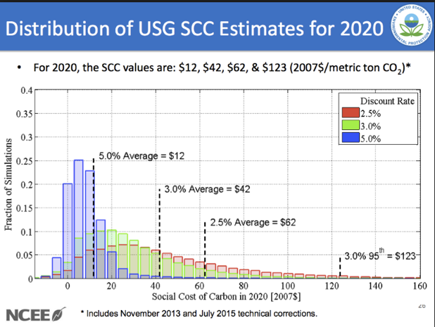
Obama Admin: $45
Uses a 3% discount rate; includes global costs
Trump Admin: less than $6
Uses a 7% discount rate; only includes American costs
PV of $1 Trillion in 2100:
$86B for Obama, $4B for Trump
Risky Assets and Optimal Portfolio Theory
Two Kinds of Optimization
Tradeoffs between two goods
Optimal quantity of one good
🍎
(not feasible)
(feasible)
🍌
Optimal choice
🙂
😀
😁
😢
🙁
🍎
benefit and cost per unit
Marginal Cost
Marginal Benefit
Optimal choice
Tradeoffs between two goods
Optimal quantity of one good
Checkpoint 1: April 20
Model 1: Consumer Choice
Model 2: Theory of the Firm
Checkpoint 2: May 4
WEEK 1
WEEK 2
WEEK 3
Modeling preferences with multivariable calculus
Constrained optimization when calculus works
Constrained optimization when calculus doesn't work
WEEK 4
WEEK 5
Consumer Demand
Applications: Financial Economics
Checkpoint 3: May 18
Final Exam: June 5
WEEK 6
WEEK 7
WEEK 8
Production and Costs for a Firm
Profit Maximization
When markets work
WEEK 9
WEEK 10
When markets need a little help
When markets fail